Visual models — 20 Watts Was Enough

lusoris contributors

These plots turn recurring equations into inspectable boundaries. They are not result figures: no curve contains workstation measurements. The equations come from the canonical math and concept notes; normalized sweeps, analytical fixture models, and explicitly hypothetical ledgers make their consequences visible before an implementation exists.

Finite-error erasure boundary

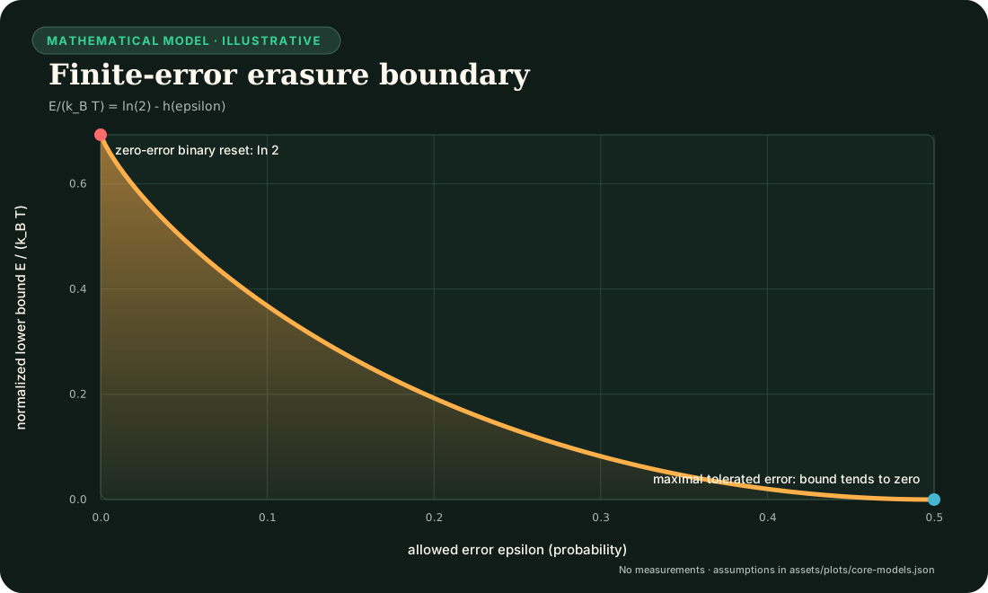
The normalized generalized erasure lower bound falls from ln 2 at zero error to zero at one-half allowed error.

For a uniform binary reset with tolerated error $\epsilon$ ,

\frac{E_{\mathrm{fund,reset}}}{k_B T} =\ln 2-h(\epsilon), \qquad h(\epsilon)=-\epsilon\ln\epsilon-(1-\epsilon)\ln(1-\epsilon).

The plot shows why $k_B T\ln 2$ is not a universal energy-per-operation constant. Relaxing the logical error changes the lower bound, while correction, retry, retained side information, duration, and downstream harm remain outside this curve. See the full derivation.

Finite-time adiabatic crossover

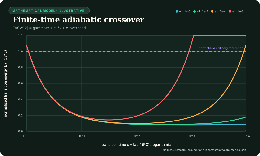
Four normalized adiabatic energy curves form different U-shaped crossovers as leakage changes.

The normalized diagnostic model is

\frac{E_{\mathrm{ad}}}{CV^2} =\frac{\gamma}{x}+\ell x+e_{\mathrm{overhead}}, \qquad x=\frac{\tau}{RC}.

Slowing a transition reduces the first term but increases leakage exposure. The minimum therefore occurs at a finite duration, and a real advantage exists only where the complete curve beats a matched ordinary reference. The plotted $\ell$ and overhead values are illustrative, not device coefficients. See the device-boundary model.

Sparse/locality break-even plane

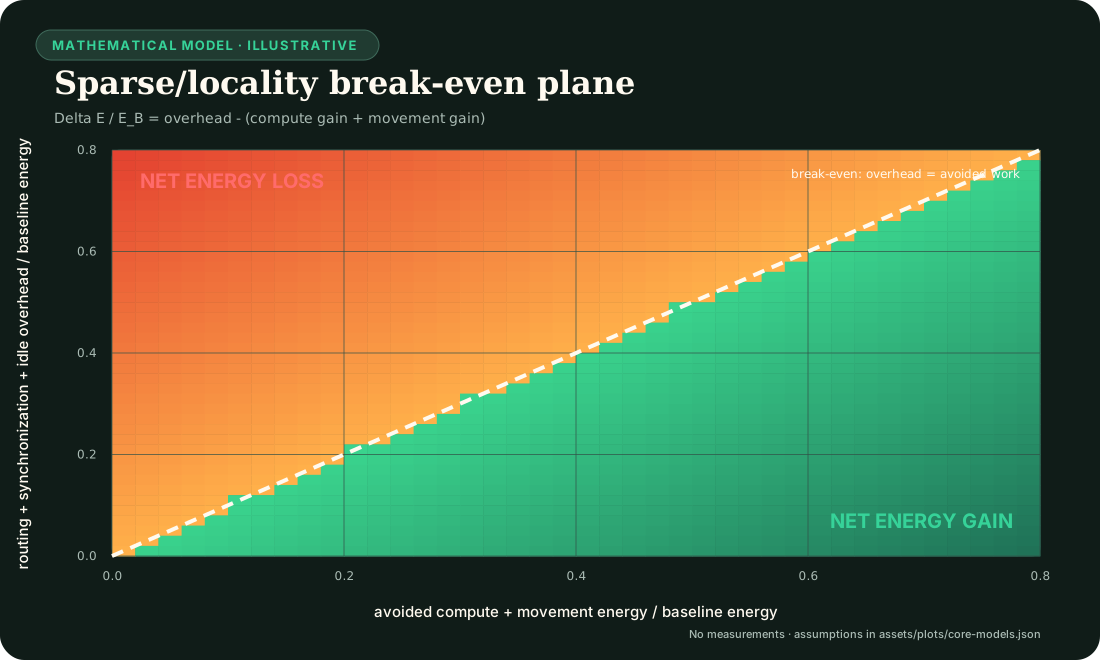
A two-color break-even plane separates net energy gain from net loss at the line where overhead equals avoided work.

Normalize all candidate-minus-baseline energy changes by baseline energy. Let $g$ be avoided arithmetic plus avoided movement and $o$ be added routing, synchronization, metadata, conversion, and idle burden. Then

\frac{\Delta E}{E_B}=o-g.

Sparse activation is beneficial only below the diagonal. A lower active parameter count on its own says nothing about which side of the boundary an implementation occupies. The underlying event ledger is defined in the energy model.

Lifecycle break-even horizon

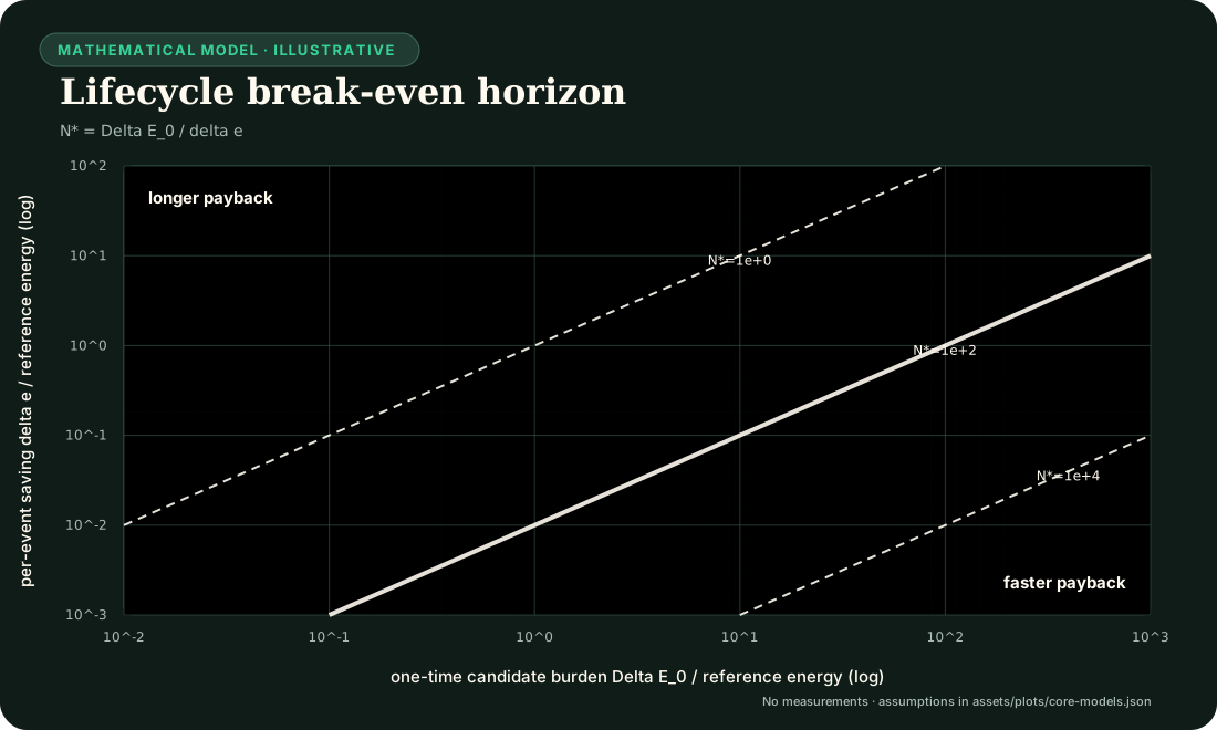
A logarithmic heatmap shows the event count needed to repay one-time candidate burden at different per-event savings.

For candidate one-time burden $\Delta E_0$ and accepted-service saving $\delta e=e_B^{\mathrm{serve}}-e_C^{\mathrm{serve}}$ ,

N^*=\frac{\Delta E_0}{\delta e}, \qquad T^*=\frac{N^*}{\lambda_q}.

The contour map makes a common failure explicit: a component can save energy per event but never repay compilation, search, fabrication, migration, or qualification within its useful service horizon. If $\delta e\leq0$ , no positive break-even exists. See the lifecycle accounting rule.

Memory-kernel truncation boundary

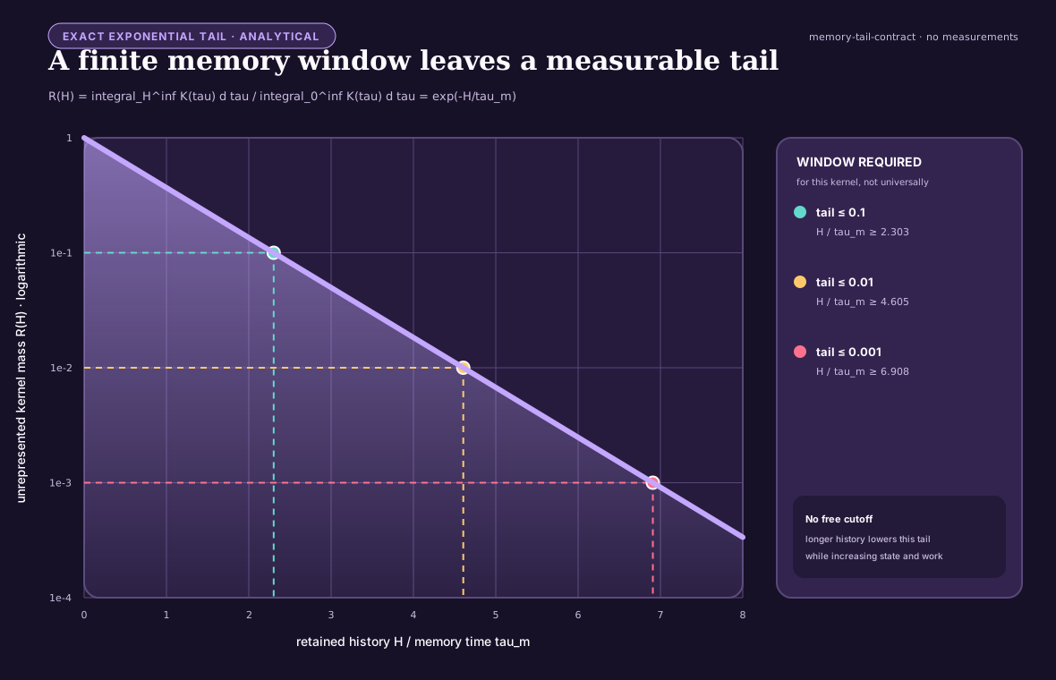
For an exponential memory kernel, the unrepresented tail falls exponentially while every tighter tolerance requires a longer retained history.

For the illustrative normalized kernel $K(\tau)=K_0\exp(-\tau/\tau_m)$ , the fraction beyond a retained window $H$ is

R(H)= \frac{\int_H^\infty K(\tau)\,d\tau} {\int_0^\infty K(\tau)\,d\tau} =\exp\!\left(-\frac{H}{\tau_m}\right).

The curve makes the storage--approximation trade explicit for this one kernel: one, two, and three decimal places of remaining tail mass require progressively longer histories. It does not supply a cutoff for another kernel, observable, horizon, or intervention. Those require an empirical closure test under the multiscale reduction contract.

Finite diffusion boundary turnover

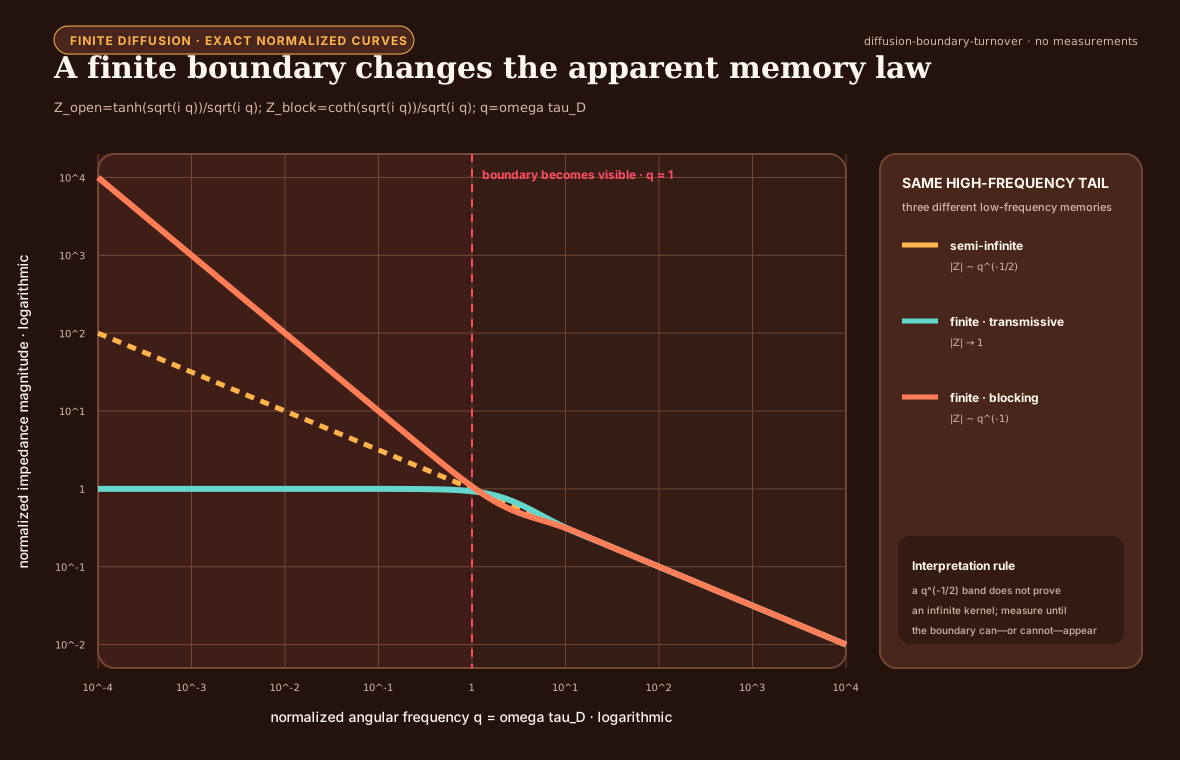
A semi-infinite diffusion law and two finite-boundary laws coincide in their high-frequency slope but separate below the boundary timescale.

Let $q=\omega\tau_D$ be dimensionless angular frequency and use normalized linear diffusion impedances

Z_{\infty}(q)=\frac{1}{\sqrt{iq}},\qquad Z_{T}(q)=\frac{\tanh\sqrt{iq}}{\sqrt{iq}},\qquad Z_{B}(q)=\frac{\coth\sqrt{iq}}{\sqrt{iq}}.

$Z_T$ is the displayed transmissive finite-boundary form and $Z_B$ the blocking form. All three have the same $q^{-1/2}$ magnitude slope at high frequency. Below $q\approx1$ , $|Z_T|$ approaches a constant while $|Z_B|$ grows as $q^{-1}$ . The exact normalized curves therefore visualize the identification problem in C-1531: a finite observation band can make physically different memory supports look alike. The curves are not fitted data and do not prescribe an artificial memory kernel.

Hysteretic memory loop

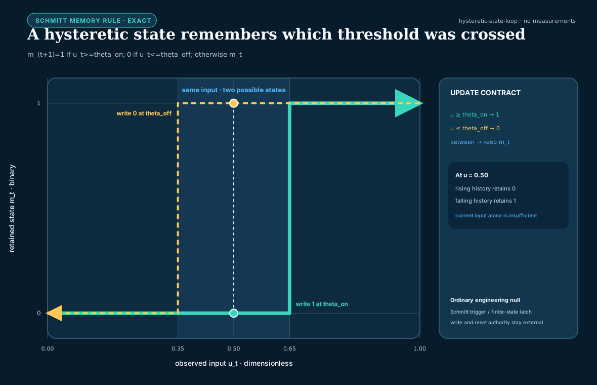
For a binary Schmitt rule, rising and falling input histories form a loop; an input inside the threshold band is compatible with either retained state.

For ordered dimensionless thresholds $\theta_{\mathrm{off}}<\theta_{\mathrm{on}}$ , the exact update rule is

m_{t+1}= \begin{cases} 1, & u_t\geq\theta_{\mathrm{on}},\\ 0, & u_t\leq\theta_{\mathrm{off}},\\ m_t, & \theta_{\mathrm{off}}<u_t<\theta_{\mathrm{on}}. \end{cases}

$u_t$ is the current input and $m_t\in\{0,1\}$ is the retained state; both are dimensionless in this normalized example. The shaded band is not uncertainty: it is the region in which history is required to determine the next state. The displayed thresholds are illustrative. The rule is included as a mature engineering null for population, analogue, or biological-memory translations, and it grants no authority to reset a state. That separate lifecycle boundary is specified in Budgeted memory lifecycle.

Slow-manifold fold boundary

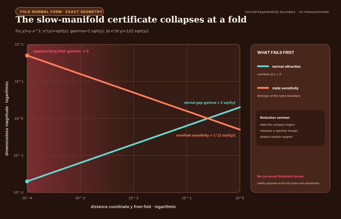
In the fold normal form, the attracting spectral gap falls to zero while the slow-state sensitivity diverges.

For the dimensionless fast equation $f(x,y)=y-x^2$ , the attracting critical branch for $y>0$ is $x^*(y)=\sqrt y$ . Its normal attraction margin and local sensitivity are

\gamma(y)=\left|\partial_xf(x^*(y),y)\right|=2\sqrt y, \qquad \left|\frac{dx^*}{dy}\right|=\frac{1}{2\sqrt y}.

As the fold at $y=0$ is approached, ordinary normal hyperbolicity disappears at the same time that a small change in $y$ produces an increasingly large change in the reduced state. The plot is an exact property of this normal form, not a universal abstention threshold. The full validity conditions are kept in the multiscale reduction contract.

Phase-selective preservation and release

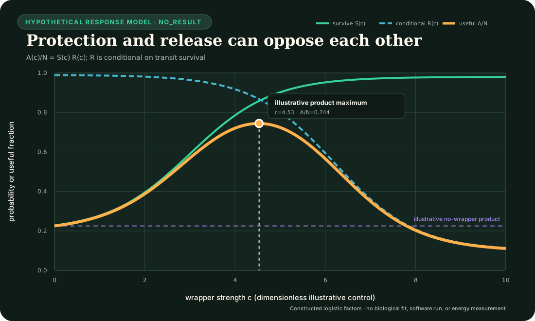
An illustrative protection factor rises with wrapper strength while release falls, so their product has an interior maximum rather than improving monotonically.

Fixture F-029 separates survival during a hostile transition from release for later service. The plotted reading aid uses the explicitly constructed logistic factors

S(c)=s_0+\frac{s_1-s_0}{1+\exp[-a(c-c_S)]},

R(c)=r_0+\frac{r_1-r_0}{1+\exp[b(c-c_R)]}, \qquad A(c)=N\,S(c)R(c).

$c$ is a dimensionless illustrative wrapper-strength control; $S(c)$ is transit survival probability; and $R(c)=P(\text{released and active}\mid\text{survived transit},c)$ is the conditional destination release-and-activation probability. Both are dimensionless. $s_0,s_1,r_0,r_1$ are dimensionless bounds; $a$ and $b$ are inverse-strength slopes; $c_S$ and $c_R$ are dimensionless midpoints; $N$ is attempted artifacts per second; and $A(c)$ is useful released artifacts per second. The figure displays $A(c)/N$ .

Increasing $c$ can improve survival while simultaneously making release less likely. A one-axis "stability" score would therefore hide the actual service failure. The chosen logistic forms and every parameter are hypothetical: they are not a fit to a protein, medicinal product, model, compiler or workstation. The useful question is whether a measured artificial implementation exhibits a support region that survives package/validation, retry, replication, reload and recompilation nulls under the complete F-029 contract.

Contextual analytical figures

The next figures are embedded where their equations first matter in the book; this index keeps their editable model and evidence status discoverable without duplicating every full-size image here.

Simultaneous Pareto decision. Illustrative uncertainty regions in relative lifecycle energy and task-native quality, with latency, risk, and support retained as hard gates. First used in Biology is a launchpad.
Costed active-acquisition frontier. A hypothetical action ledger for $\Delta U-\lambda_EE-\lambda_LL-\lambda_BB$ after risk and latency admissibility. First used in Sparse prediction and adaptive compute.
Recovery-time fragility curve. Exact evaluation of the Candidate 003 linear-simulator equation $\tau_{95}=\Delta t\ln(0.05)/\ln(g)$ with its declared illustrative Stage-1 threshold. First used in Maturity and structural consolidation.
Memory-action price envelope. Hypothetical single-item lines $G_a-\lambda_EE_a$ and their admissible upper envelope. First used in Fast memory, replay, and consolidation.
Mission-profile damage history. Two constructed equal-mean temperature histories passed through one hypothetical Arrhenius-rate model. First used in Reliability under mission profiles.
Fixture F-007 identifiability. Analytical likelihoods that coincide under a base operator and separate after an added measurement. First used in Operator-qualified sensing.
Interface-qualified scale symmetry. Two exact geometrically scaled paths produce the same $y=\ln(u/r)$ trajectory in a positive-domain reference model while a separate illustrative absolute gate distinguishes them. First used in Interface-qualified scale symmetry.
Interface-qualified retroactivity. A paired isolated/connected mass-action trajectory is plotted above the exact reduced retroactivity factor across load and operating point. The parameters are hypothetical and the figure reports neither delivered service nor energy. First used in Interface-qualified retroactivity.
Phase-selective preservation and release. Constructed opposing survival and release factors whose product has an interior maximum. The figure introduces no measurement or optimum and is defined above for Fixture F-029.

Every value in these figures is labeled analytical or illustrative. None is a workstation result, a promoted claim, or a recommended deployment threshold.

Reproduction and editing

The editable parameter source is core-models.json. The deterministic generator is scripts/generate-plots.mjs; generated SVG files live under public/plots/. Change the specification or generator, regenerate, and commit source and output together.