Skip to first chapter

Research portal

20 Watts Was Enough — Full Concept Book

The complete public reading edition generated from canonical Git source.

Edition
Site v0.3.0 · continuous main snapshot
Source revision
ec2865b0eac15148675c629981a545632b3571c5
Source
Git main snapshot

Project · 1,201 words

20 Watts Was Enough

CI GitHub Pages OpenSSF Scorecard Latest release Code: EUPL 1.2 Original content: CC BY-SA 4.0

A biologically inspired R&D blueprint for sparse, grounded, continual, energy-efficient AI.

The adult human brain operates within a whole-organ power budget of roughly 17–20 watts (C-001). That observation does not provide a fair brain-versus-silicon benchmark by itself; it establishes a serious engineering question: which computational constraints behind adaptive biological intelligence can be translated into measurable requirements for artificial systems? The energy evaluation chapter defines the boundary required for a comparison.

This repository turns that question into a traceable research programme: primary evidence becomes scoped claims, cross-domain mechanisms are deduplicated, and retained ideas face explicit null models and failure rules.

Current status: the evidence framework, architecture and bounded experiment machinery exist. An integrated AI system and claim-eligible workstation result do not. Development smoke checks remain NO_RESULT. The generated coverage report and readiness summary record the exact current boundary.

Read the project

GoalStart here
Understand the question and proposed systemWorking architecture
Browse the research onlineResearch portal
Read continuouslyFull HTML book
Read offline or printDownload the A4 PDF
Inspect evidenceClaim ledger and bibliography
Inspect the plan and proposed testsResearch roadmap and experiment coverage
Run a released experiment imageContainer execution contract
Help with a bounded taskPublic contribution map
Find a specific areaRepository map

The portal and web book list all 24 official EU languages, but publish only translations tied to an exact canonical source digest and human review. English remains canonical. Where a reviewed translation does not yet exist, the language control opens a focused contribution issue instead of unlabelled machine output. See the translation contract.

What the project tests

Useful adaptive intelligence may require much less active computation and data movement than current systems routinely spend. The project investigates whether that gap can be attacked through a system that:

  • separates total capacity from active capacity;
  • grounds representations in aligned perception, action, and outcome;
  • allocates computation according to uncertainty and task demand;
  • separates rapid episodic learning from slow structural learning;
  • consolidates before pruning or hardening;
  • keeps mutable facts in inspectable memory rather than forcing everything into weights; and
  • measures quality, energy, data movement, lifecycle cost, and uncertainty together.

Nature is a source of mechanisms, not a shortcut around engineering controls. Observations from neuroscience, biology, ecology, physics, chemistry, mathematics, social systems, and other fields are normalized by their causal operation, deduplicated into shared principle bundles, and tested against strong ordinary engineering alternatives.

Plan and progress

The research roadmap is the canonical dependency order. Its stages run from evidence and experiment contracts through isolated mechanisms, adaptation, grounding, structural maturation and substrate co-design. They are gates, not promised dates.

GitHub milestones project those stages into issues and pull requests. They answer what work is open and who is doing it; they do not decide whether a scientific claim is established. The authorities remain separate:

QuestionAuthority
What should happen next?Research roadmap
Which bounded tasks are open or finished?GitHub milestones projected from the milestone manifest and repository-bound issue map
What does the evidence support?Claim ledger
Which experiment paths are actually ready?Coverage report and readiness summary

Closing an issue updates operational progress. Only a reviewed evidence change updates a claim, and only a qualifying run updates result status.

The default normative context is the European Union and Germany. Legal, standards, and conformity statements remain qualified by jurisdiction, role, version, applicability, and date under the normative baseline.

Scientific conduct follows the research integrity baseline, which deduplicates the recurring ALLEA, EU, DFG, and large European university rules for disclosure, stewardship, ethics, correction, and review.

How the repository works

primary sources -> scoped claims -> deduplicated principles
                -> engineering translations -> equations and architecture
                -> equal-budget tests -> bounded evidence -> revised claims
  • research/claims.md gives major assertions stable C- identities and evidence status.
  • research/principle-registry.md groups equivalent cross-domain mechanisms under stable P- identities.
  • concept/ develops the maintained system synthesis.
  • math/ defines notation, units, derivations, and testable efficiency models.
  • experiments/ separates written protocols, development plumbing, and result authority.
  • decisions/ records durable choices without rewriting their history.
  • sources/ preserves provenance and publication boundaries; imported discussions and summaries are leads, not evidence.

Canonical source and editing

Git main is the canonical source. The Pages portal, HTML book, and PDF are generated views of the same committed material; Google Docs and imported chats are not synchronized document stores. Work incrementally on one chapter, claim, equation, diagram, test, or decision rather than regenerating the whole project.

Read AGENTS.md and the engineering and research contract before editing. The research-writing skill keeps project prose direct and evidence-aware, with a deliberately narrow automated check for high-confidence generated filler. The repository-rule crosswalk explains which conventions from the maintainer's other projects were adopted, adapted, staged, or rejected here.

For a local live preview:

npm ci
npm run dev:github-pages

The preview runs at http://localhost:5173/ and reloads canonical Markdown, equations, tables, diagrams, and plots as their source files change.

Qualifying releases publish repository tooling and individual experiments as small container images. Use the complete image@sha256:... identity from the release's checksum-bound oci-images.json, not a mutable tag. The release contract explains admission, provenance and supported platforms; the experiment instructions provide the exact isolated commands. For example, the static validation image runs without network access:

image='ghcr.io/lusoris/20-watts-was-enough-20w@sha256:...'
docker pull "$image"
docker run --rm --network none \
  --pull never \
  --mount "type=bind,src=$PWD,dst=/repo,readonly" \
  "$image" \
  validate docs --root /repo

Releases may also attach a verified native Go binary as a convenience. The containers are the portable public default and remain scoped per experiment.

Before a local commit, follow the validation sequence: check the changed contracts and their downstream consumers, combining scopes for mixed changes. Unknown, unsafe or shared-authority scope requires the full gate.

Run the complete npm and Go gates before marking a pull request ready, integrating into main, merging or releasing.

Changes to book sources also require:

npm run generate:book-pdf
npm run validate:book-pdf

See CONTRIBUTING.md for the complete workflow and SUPPORT.md for issue routing. The repository does not maintain a PowerShell, C# or host-specific execution lane.

Citation, support, and licence

Use CITATION.cff and identify the exact release or commit when citing the project. Scientific use should also cite the original sources that support the specific claim; citing this synthesis does not replace them.

If the project is useful, support is available through Ko-fi or GitHub Sponsors.

Project-authored software, scripts, tests, configurations, schemas, and workflows are licensed under the EUPL v1.2 or later. Original project prose, mathematics, diagrams, plots, and presentation are licensed under CC BY-SA 4.0. Third-party and source material retains its own terms. Read LICENSING.md for the controlling boundary.

Concept · 668 words

Thesis and design principles

Scope

This chapter states the project's argument, its engineering requirements, and the limits that keep a biological analogy from becoming mythology.

Thesis

The brain demonstrates that adaptive behavior, continual learning, perception, memory, and action can coexist under a tight energy and communication budget (C-001). Contemporary AI demonstrates a different strength: highly parallel optimization over vast data and parameter spaces.

The project hypothesis is that a capable artificial system should combine the search capacity of modern learning with constraints that biology cannot evade:

  1. only a small, relevant fraction of capacity should be active for an event;
  2. communication and memory movement must be priced, not hidden behind FLOPs;
  3. learning must begin from aligned perception, action, and consequence rather than language alone;
  4. rapid acquisition must not directly rewrite stable long-term structure;
  5. consolidation must precede destructive compression; and
  6. stable skills, mutable facts, and active reasoning should use different storage and execution paths.

The intended result is a system whose cost scales primarily with the information and uncertainty relevant to a task, rather than with its full stored capacity.

Biological observation

Neural signaling is metabolically costly, cortical activity is constrained, and biological learning spans multiple timescales. Sensory and motor experience precedes mature language. These observations motivate design constraints.

They do not establish a single brain algorithm, an equivalent number of digital operations, or a guarantee that every biological mechanism is efficient on silicon.

Proposed AI translation

The blueprint combines four separations:

  • capacity versus activity: sparse routers select modules, depth, memory, and precision;
  • prediction versus correction: predictable state follows a cheap path; residual uncertainty receives more computation;
  • experience versus structure: fast memory captures episodes while slow learning integrates regularities under regression tests; and
  • reasoning versus knowledge: stable skills may be compiled or quantized, while mutable facts remain retrievable and attributable.

Development is a controlled lifecycle:

flowchart LR
    seed["Capacity-rich modular seed"] --> ground["Sensorimotor grounding"]
    ground --> plastic["Sparse active learning"]
    plastic --> consolidate["Replay and consolidation"]
    consolidate --> validate["Generalization and stability gates"]
    validate --> prune["Structured pruning"]
    prune --> harden["Quantize, compile, or externalize"]
    harden --> operate["Continual operation"]
    operate --> plastic

Editable source: ../assets/diagrams/developmental-pipeline.mmd.

Efficiency mechanism

The optimization target is constrained quality per unit of total system energy, with latency and uncertainty limits. A model is not efficient merely because it has sparse weights; the runtime must avoid loading and operating on inactive state, and routing overhead must remain smaller than the work skipped.

The top-level objective is developed in the energy model:

max  QEfacilitysubject toLp95Lmax,  RRmax,  QQmin.\max \; \frac{Q}{E_{\text{facility}}} \quad \text{subject to} \quad L_{p95} \le L_{\max},\; R \le R_{\max},\; Q \ge Q_{\min}.

Here QQ is task quality, EfacilityE_{\text{facility}} is measured facility energy, Lp95L_{p95} is tail latency, and RR is a defined risk or calibration metric.

Evidence status

  • Metabolic constraints on neural activity are established within the scope of C-001.
  • Conditional computation is established in narrower engineered systems under C-003 and C-004.
  • The complete developmental pipeline is a speculative integration. No cited paper validates it as one system.

Speculative extensions

  • Learn a global energy price that modules must “bid” against when requesting compute.
  • Let stable routing motifs become physically colocated or compiled for lower data-movement cost.
  • Allow controlled structural growth when no existing module can absorb a new regime without interference.

Failure modes

  • Anthropomorphic labels conceal incompatible mechanisms.
  • Sparsity saves theoretical FLOPs but increases real communication or latency.
  • Energy optimization suppresses rare but important computation.
  • Early specialization prevents transfer and produces brittle modality silos.
  • “Hardening” turns uncertain or mutable behavior into an uncorrectable path.

Measurable predictions

The integrated hypothesis survives only if, at matched quality:

  • active parameters and memory traffic grow more slowly than total capacity;
  • average energy falls without unacceptable tail-risk or calibration loss;
  • sequential learning retains prior capability better than a matched single-timescale baseline; and
  • grounded intervention tasks improve beyond gains explained by additional data or parameters alone.

Concept · 2,359 words

Working architecture: three coupled loops

A capable system should execute, adapt, and consolidate on different timescales while one controller prices energy, latency, and risk.

Scope

This is the shortest complete description of the proposed system. It joins the project's individual mechanisms into one operating architecture and shows where information moves, where learning happens, and which decisions remain reversible.

Architecture at a glance

flowchart TB
    subgraph event["Event loop"]
        direction LR
        world["World · user · tools"] --> fast["FAST RUNTIME<br/>predict · select · execute"]
        fast --> result["Outcome + telemetry"]
        result --> world
    end
    subgraph lifecycle["Learning and lifecycle"]
        direction LR
        adapt["ADAPTATION"] --> provisional["Episodes + provisional modules"]
        provisional --> slow["MAINTENANCE"]
        slow --> stable["Slow model + hardened paths"]
    end
    result --> adapt
    provisional --> fast
    stable --> fast
    budget["Resource + risk controller"] -. "energy · latency · risk" .-> fast
    budget -.-> adapt
    budget -.-> slow
    result --> budget

Editable source: ../assets/diagrams/three-coupled-loops.mmd.

The three loops solve different problems:

LoopTimescalePrimary decisionNormal output
Fast runtimeeventWhat should run now?action, answer, or escalation
Adaptationepisode to sessionWhat did this outcome teach us?attributable episode, hypothesis, or provisional module
Maintenancereplay to release cycleWhat should become stable, move, weaken, or disappear?consolidated memory and restructured execution

The resource controller crosses all three. It can restrict an action because of energy, latency, communication, or risk, but it cannot silently replace the task objective. Measured outcomes return to the controller so estimated costs can be corrected.

Biological observation

Living systems repeatedly separate processes by timescale and locality:

  • many components are available, while only a small subset is strongly active together (C-001, C-003);
  • local circuits resolve routine events while larger systems coordinate exceptions (C-017, C-024);
  • fast traces change behavior before slow structure is rewritten (C-008, C-019);
  • replay, forgetting, and structural maintenance are selective processes (C-036C-042);
  • stable structure can be protected and later reopened under bounded intervention (C-043C-045); and
  • local demand can recruit adjacent resource supply (C-049C-051).

The shared principle is separation of concerns: execution, adaptation, memory, structure, and physical supply change at different speeds and respond to different signals. Digital systems add exact copying, external stores, checkpoints, shadow evaluation, and rollback. Those capabilities make the separations easier to test and safer to revise.

Proposed AI translation

1. Fast runtime

For each event, the runtime forms a predictive state containing expected observations, uncertainty, current goals, and relevant recent context. A hierarchical selector then chooses the cheapest admissible path:

  • a hardened low-cost path for a familiar, low-risk event;
  • one or more conditionally active experts;
  • another layer or reasoning step;
  • episodic or factual retrieval;
  • a sensor, tool, or environment intervention; or
  • escalation to a human or a more capable controller.

The output is more than an answer. It includes measured latency, energy, communication, calibration, and any observed consequence. That telemetry is the input to later learning and resource decisions.

2. Adaptation

An outcome is captured with provenance before it can alter slow parameters. It may update temporary state, create a provisional adapter, change a local connection, or simply become a replay candidate. A surprising event is not automatically a lesson; it may be noise, attack, contradiction, or evidence of a new regime.

There is no ex-nihilo generator in this design. Every proposal is built from inherited structure and experience: complete patterns, fragments, relations, or abstractions are copied and transformed. The generative cycle is therefore explicit:

flowchart TB
    sources["Inherited structure + experience"] --> copy
    subgraph synthesis["Construct a candidate"]
        direction LR
        copy["Copy fragments + relations"] --> compress["Compress + abstract"]
        compress --> vary["Vary + recombine under a goal"]
    end
    vary --> test{"Test in simulation or the world"}
    subgraph selection["Evaluate the result"]
        direction LR
        test -->|"supported"| retain["Retain with provenance"]
        test -->|"fails"| revise["Reject · revise · keep uncertain"]
    end
    retain --> sources
    revise --> vary

Editable source: ../assets/diagrams/generative-recombination.mmd.

Stochasticity can alter which variants are tried. Usefulness comes from the entire cycle: decomposition, recombination, intervention, comparison, and selection. The supporting evidence and unresolved distinctions are tracked in the endogenous generation audit and is falsified first through Candidate 004.

Reconstructive adaptation through external state

Visual art and design cognition make the cycle more operational. Proposal generation is reconstructive: learned categories, exemplars, relations, styles, constraints, tools, and prior transformations shape what can be proposed (C-842C-860). That does not reduce the process to nearest-neighbor retrieval. A system can externalize a partial state, inspect consequences that were not explicit in its preceding plan, change representation, probe the world, and use the result to create a new branch. The novelty is relative to a declared history; the validity comes from constraints and observed outcomes.

The adaptation loop therefore distinguishes seven event types:

  1. Exposure: which sources, examples, styles, and constraints were available before the task;
  2. Retrieval: which versioned sources were deliberately requested during the task and at what cost;
  3. Reconstruction: which fragments, relations, or abstractions formed a proposal branch;
  4. Externalization: which editable representation—text, sketch, scene graph, CAD state, program, simulation, or prototype—made the proposal inspectable;
  5. Epistemic action: which render, measurement, simulation, query, or material intervention was selected to reduce a decision-relevant uncertainty;
  6. Evaluation and selection: which hard constraints, qualified evaluators, risk limits, and selection rule admitted or rejected a version; and
  7. Retention: which source, parent, operation, test, rejected branch, dependency, expiry, and rollback records were preserved.
flowchart LR
    brief["Hidden problem · declared constraints · evaluator contract"] --> expose["Logged source exposure"]
    corpus["Versioned source corpus"] --> expose
    corpus --> retrieve["Metered retrieval · precedents · cases"]
    expose --> reconstruct["Reconstructive generation"]
    retrieve --> reconstruct
    reconstruct --> branches["Independent proposal branches"]
    branches --> externalize["Externalize · sketch · scene graph · CAD"]
    externalize --> inspect["Inspect · query · resegment"]
    inspect --> transform["Transform representation or proposal"]
    transform --> externalize
    inspect --> action["Epistemic action · render · simulate · probe"]
    action --> material["Material or environment feedback"]
    material --> externalize
    externalize --> diversity["Diversity and fixation audit"]
    diversity --> evaluate["Constraint validity · usefulness · risk · cost"]
    evaluate --> select["Blinded evaluation and selection"]
    select --> retain["Retain · expire · recombine · rollback"]
    retain --> lineage["Version graph · sources · operations · tests · rejected branches"]
    lineage --> retrieve
    nulls["Retrieval · CAD/editors · diffusion · QD/BO · scratchpads · active learning"] --> evaluate

Editable source: versioned-reconstructive-design.mmd.

Several separations are non-negotiable. More proposals are not necessarily better proposals; proposal diversity, constraint validity, selection regret, and realized outcome are different measurements. Similarity to an example can transfer a useful structural relation or cause fixation and negative transfer, so similarity and task effect are both reported. A provenance graph can record derivation without proving intention, authenticity, correctness, or originality. Aesthetic response is observer-, context-, expertise-, and history-qualified rather than a universal scalar.

Parallel branches are useful only if they remain genuinely independent before critique. A shared canvas can coordinate work and simultaneously propagate an early fixation. The comparison therefore includes private branches, delayed reveal, source substitution, example removal, evaluator swap, material swap, and representation conversion. Every alternative pays for retrieval, proposals, tools, simulations, human critique, physical material, waste, retention, and recovery.

Fixture F-002 tests this complete loop against a mature composition of retrieval, CAD and editors, generative sampling, explicit search and quality-diversity, scratchpads and shared workspaces, active learning, simulation, version control, provenance, and independent reranking. The mathematical contract keeps exposure, retrieval, relative novelty, reinterpretation, information gain, fixation, negative transfer, constraint margins, evaluator qualification, selection regret, lineage, reconstructability, and lifecycle cost separate. If that ordinary stack ties, the additional architecture is removed while the fixture remains as a negative result.

3. Maintenance

Maintenance receives a budgeted set of possible actions. For any memory, module, or route it may:

  • defer while collecting more evidence;
  • replay against related and conflicting cases;
  • merge redundant records while retaining provenance;
  • externalize mutable propositions to an inspectable store;
  • reduce influence or plasticity;
  • delete state after retention and safety checks;
  • reopen mature structure in a reversible branch;
  • change logical topology or physical placement; or
  • promote stable computation into a cheaper representation.

The formal action model is defined in ../math/memory-lifecycle.md. Structural changes remain shadowed and reversible until regression, calibration, and energy tests pass.

4. One event end to end

  1. A sensor, user, or tool changes the current state.
  2. The runtime predicts what matters and estimates uncertainty.
  3. The selector chooses depth, modules, memory, precision, and possible intervention under the current budget.
  4. Execution produces an outcome and physical telemetry.
  5. The adaptation loop stores an attributable episode and may construct a bounded hypothesis or provisional module.
  6. The maintenance loop later replays the episode against related and conflicting evidence.
  7. A validated regularity may be consolidated, compiled, quantized, externalized, relocated, or used to change future routing.
  8. Regression or fragility tests can reject the change and restore the previous state.

5. State ownership

StatePrimary ownerNormal write pathReason for separation
Current predictive stateruntimeevery eventcheap, transient, task-specific
Attributable episodesadaptationobserved outcomepreserves evidence before abstraction
Provisional hypothesesadaptationbounded generation and trialspermits novelty without global drift
Reusable skills and representationsslow modelvalidated consolidationstable transfer across events
Mutable propositionsfactual memorysourced, versioned updatecorrection, attribution, and conflict
Hardened execution pathscompiled storepromotion pipelinelower repeated interpretation cost
Lifecycle and fragility statemaintenancereplay, probes, regressionsrepair remains separate from execution
Resource and risk policycontrollercalibrated policy updatelocal mechanisms cannot hide physical cost

Efficiency mechanism

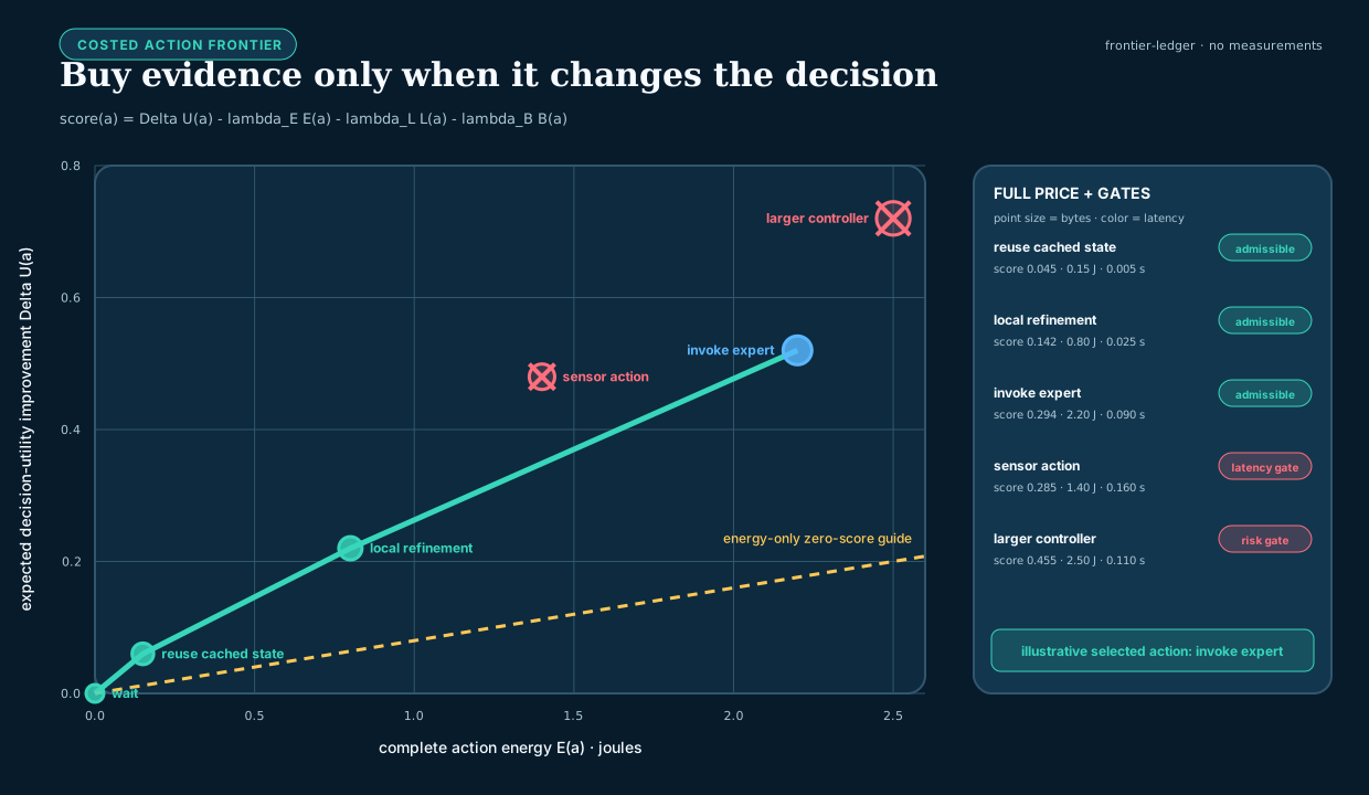
Efficiency is an event-level constrained decision. At time tt, the selector chooses an admissible action aa from At\mathcal{A}_t:

at=argmaxaAtE[ΔV(a)st]a_t^*=\arg\max_{a\in\mathcal{A}_t} \mathbb{E}[\Delta V(a)\mid s_t]

subject to

E(a)BtE,L(a)BtL,R(a)ϵtR.E(a)\le B_t^E,\qquad L(a)\le B_t^L,\qquad R(a)\le \epsilon_t^R.

Here sts_t is the predictive state; ΔV(a)\Delta V(a) is expected task-value improvement; E(a)E(a) is energy in joules; L(a)L(a) is latency in seconds; R(a)R(a) is the declared risk measure; and BtEB_t^E, BtLB_t^L, and ϵtR\epsilon_t^R are event-specific limits. Measured cost after execution recalibrates the estimator.

Lifecycle comparison includes the work usually hidden outside inference:

Elife=Erun+Ememory+Enetwork+Eadapt+Emaint+Erecovery.E_{\mathrm{life}}= E_{\mathrm{run}}+E_{\mathrm{memory}}+E_{\mathrm{network}}+ E_{\mathrm{adapt}}+E_{\mathrm{maint}}+E_{\mathrm{recovery}}.

An architecture advances only if it improves the joint frontier of quality, risk, latency, and lifecycle energy against its strongest conventional baseline. Skipped FLOPs alone are not an efficiency result.

Evidence status

ComponentCurrent evidenceTranslation status
Conditional experts and early exitC-003, C-004implemented mechanisms; physical benefit remains system-specific
Predictive residual allocationC-005–C-007, C-022plausible composition; grounded experiment required
Fast/slow memory and replayC-008–C-010, C-036–C-042scoped evidence; lifecycle controller experimental
Structural maturation and reopeningC-012, C-043–C-045biological interventions established; digital state machine speculative
External factual memoryC-014usable mechanism; conflict and energy policy unresolved
Local resource and context controlC-046–C-051biological observations established; proposed control planes experimental
Endogenous proposal generationC-061–C-066constituent observations established; integrated curriculum speculative
Versioned reconstructive designC-842–C-860constituent observations scoped; complete externalize–inspect–transform–evaluate loop unvalidated
Complete three-loop systemnoneunvalidated synthesis

The engineering analogue audit maps the architecture to feedback control, value of information, caches, schedulers, change detection, adaptive routing, replicated state, and system identification. Each experiment must compare against the strongest relevant version of those methods.

Speculative extensions

  • Receiver-specific fast and slow context channels under a hard bit budget.
  • Modules bidding for compute by expected value improvement while a global controller enforces physical and safety constraints.
  • Active fragility probes on shadows or replicas before topology changes.
  • Capability-gap repair that admits complementary modules instead of restoring arbitrary capacity.
  • Joint learning of logical routing, memory placement, and hardware locality.

Each remains outside the core architecture until its isolated contract beats the appropriate engineering baseline.

Failure modes

  • Dense control disguised as sparsity: routing, broadcast, or monitoring moves nearly as much state as dense execution.
  • Controller conflict: runtime, adaptation, maintenance, and resource loops oscillate or optimize incompatible signals.
  • False maturity: a shortcut appears stable and is hardened before compositional and intervention tests.
  • Memory laundering: unsupported episodes become slow parameters without provenance or contradiction checks.
  • Maintenance dominates cost: replay, probes, migrations, and regression testing consume the savings of conditional execution.
  • Fixation propagates through shared state: early examples or collaborators collapse independent branches before alternatives are tested.
  • Generation impersonates evaluation: the proposal model's own score is reported as independent evidence of validity or usefulness.
  • Lineage impersonates truth: a complete derivation record is treated as proof of correctness, intention, authenticity, or originality.
  • Renaming without mechanism: a familiar cache, controller, or scheduler receives a biological label without a different causal operation.

Measurable predictions

The architecture earns implementation only if isolated experiments support the following predictions:

  1. Conditional execution reduces measured data movement and wall energy at matched quality, calibration, and tail risk.
  2. Fast attributable memory improves adaptation latency while slow-model regression remains bounded.
  3. Reversible maturity gates reduce catastrophic drift without blocking necessary relearning or newcomer admission.
  4. Structured recombination plus targeted intervention produces more valid, useful novelty than matched-budget stochastic sampling alone.
  5. Editable externalization, inspection, representation change, and epistemic action improve hidden-constraint validity, selection regret, and transfer beyond the complete retrieval/editor/generation/search/tool stack without increasing fixation or lifecycle cost.
  6. Maintenance improves retention and adaptability after replay, monitoring, migration, and recovery costs are counted.
  7. At least one proposed mechanism beats the strongest ordinary controller, scheduler, cache, router, or system-identification baseline.

Until those tests pass, this is a working architecture: precise enough to reject, modular enough to simplify, and explicitly incomplete.

Concept · 1,024 words

Biology is a launchpad, not a ceiling

Scope

This chapter defines how the project may borrow from living systems without turning a biological implementation into a specification. The brain is an existence proof for efficient adaptive intelligence, but neither evolution nor neural tissue optimized the same objective, hardware, scale, or reliability contract as an artificial system.

The working rule is:

Reproduce the useful constraint or computation, not the substrate accident.

Biological observation

Biological intelligence is shaped by slow, noisy, failure-prone components; metabolically expensive communication; physical growth; local chemical signals; and an inability to checkpoint, clone, or roll back a whole organism. Brains compensate with local processing, sparse activity, redundancy, specialized cell types, multiple timescales, and continual maintenance.

Those compensations are informative, but they are not automatically optimal on silicon. Digital systems offer different capabilities: fast switching and interconnect, exact copying, explicit addressing, external storage, reversible experiments, global synchronization when it is worth its cost, and precision that can be selected per operation. At the same time, digital systems still pay heavily for data movement, memory access, communication, cooling, and idle capacity. The relevant question is which constraints and useful computations survive a change of substrate.

The speed comparison must stay qualitative until a shared task and latency boundary exist. Axonal conduction, synaptic integration, transistor switching, GPU kernels, and cluster collectives are different operations. Selecting the fastest number from each domain would recreate the invalid comparison rejected by C-016.

Proposed AI translation

For each biological candidate, record five transformations:

  1. Observed function: what the organism demonstrably achieves.
  2. Biological constraint: which physical or evolutionary limit shaped it.
  3. Candidate invariant: the computation that may survive a substrate change.
  4. Silicon implementation: the least literal engineered mechanism that tests the invariant.
  5. Escape hatch: the biological limitation that engineering should not inherit.
Biological patternCandidate invariantSilicon-native escape hatch
Mostly local signalingPrice communication and keep repeated work near its statePermit fast global exchange when its measured value exceeds its traffic cost
Slow, noisy spikesEvent-driven, uncertainty-sensitive updatesUse dense vector arithmetic or exact digital state where it is cheaper
Synaptic and dendritic computationCompute near stored state; route locally before global aggregationImplement fused kernels, hierarchical memory, or programmable modules rather than literal morphology
Sleep and replaySeparate acquisition from protected integrationConsolidate asynchronously, continuously, or from exact checkpoints
Development and pruningExplore with reversible capacity, then commit after evidenceGrow, clone, roll back, and reallocate modules without waiting for physical development
Multiple memory systemsMatch update rate and provenance to information lifetimeUse databases, caches, logs, tools, and versioned weights unavailable to animals
Homeostasis and repairTreat stability and maintenance as active control loopsUse telemetry, deterministic tests, redundancy, and replacement hardware

This transformation is a project decision, not evidence that any row will produce a gain. The candidate inventory is maintained in the neuroscience opportunity map and comparative-biology map. Its relationship to existing AI is tracked in the adoption matrix.

Efficiency mechanism

The approach preserves useful functions in the cheapest available form and uses digital capabilities—including exact copies, reversible branches, and direct addressing—where they improve the measured system.

For a biological candidate mm, the engineering experiment compares at least three systems: a conventional baseline BB, a literal or close biological translation LmL_m when meaningful, and a silicon-native abstraction SmS_m. Using the measurement contract from the energy model, the candidate is interesting only if SmS_m improves the quality–risk–energy frontier:

(Q,R,E,L)Sm(Q,R,E,L)B,(Q, R, E, L)_{S_m} \succ (Q, R, E, L)_B,

where QQ is task quality, RR is the declared risk metric, EE is energy within the declared boundary, and LL is latency. The symbol \succ means Pareto dominance under pre-registered tolerances; it does not collapse unlike units into a decorative score.

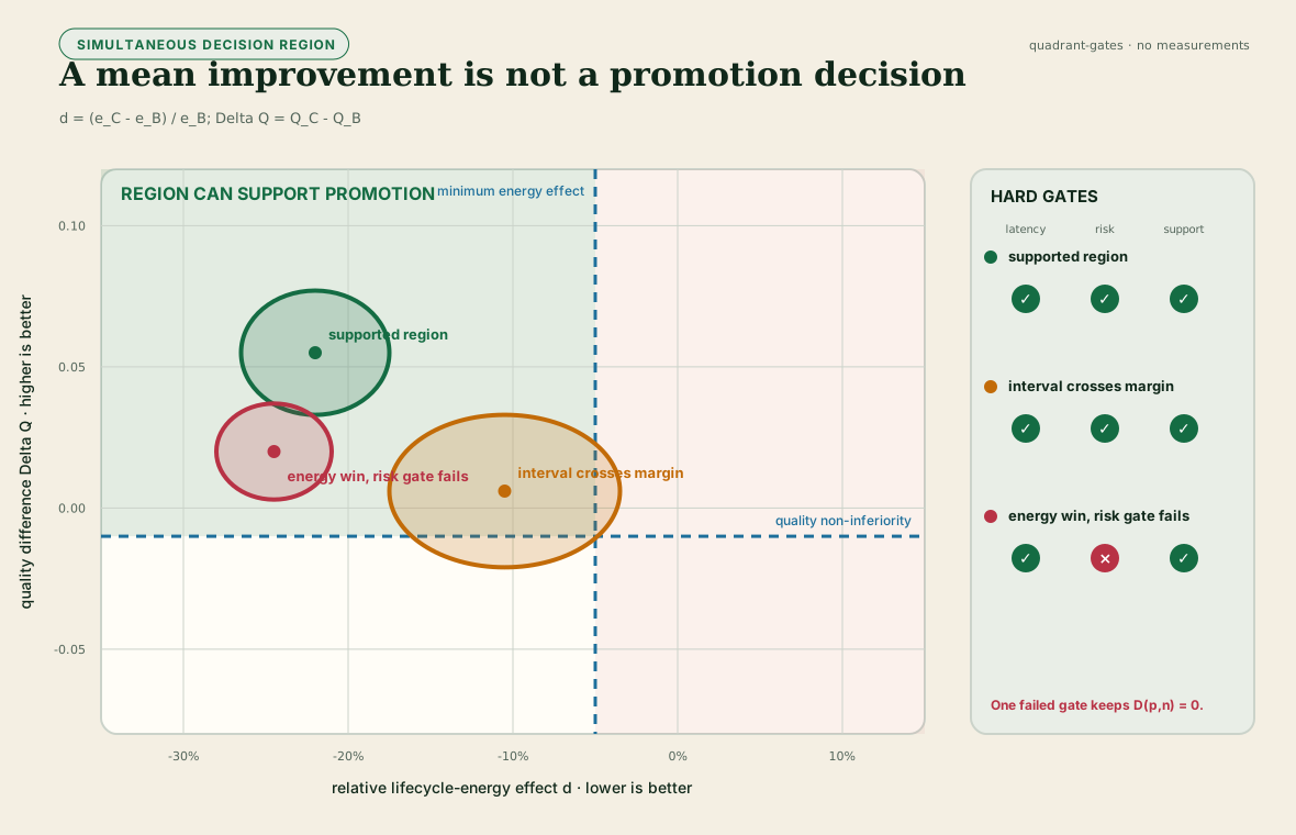
The decision geometry below is illustrative. Its points and simultaneous regions are not measurements; they show why a favorable mean on one coordinate cannot override uncertainty or a failed protected-outcome gate.

A favorable mean energy difference is insufficient: promotion requires the entire simultaneous uncertainty region to clear the energy and quality margins while every risk, latency, and support gate remains valid.

Evidence status

  • Neural energy constraints are established only within the scope of C-001.
  • Nonlinear dendritic subunits, homeostatic scaling, neuromodulated plasticity, and specialized inhibitory control are biological observations under C-017 through C-020; their proposed artificial abstractions are not thereby validated.
  • Performance of the complete cross-substrate system remains speculative until matched engineering tests establish it.

Speculative extensions

  • Learn when global communication is worth buying instead of banning it.
  • Compile frequently reused local circuits into fast deterministic paths while retaining a slower plastic path for exceptions.
  • Search jointly over algorithm, memory hierarchy, interconnect, precision, and physical embodiment rather than treating hardware as a final deployment detail.
  • Import organizational principles from organisms without centralized brains, including plants, immune systems, cephalopod limbs, and adaptive transport networks.

Failure modes

  • A metaphor is mistaken for a mechanism.
  • “Biological” becomes an unearned synonym for efficient or intelligent.
  • “Silicon is faster” is used to ignore memory movement, synchronization, or thermal limits.
  • A negative result for one implementation is treated as falsifying the underlying biological abstraction—or vice versa.
  • The project claims an idea is absent from AI after finding only that it is absent from mainstream foundation models.
  • Evolutionary fitness is confused with task accuracy, truthfulness, or human values.

Measurable predictions

This framing earns its place if, across isolated mechanism experiments:

  • silicon-native abstractions equal or outperform literal translations at matched quality and system boundary;
  • retained biological constraints predict where energy or interference is saved;
  • removing a proposed invariant removes the benefit even when the biological surface form remains; and
  • at least one hybrid uses a capability unavailable to biology—such as exact rollback or external versioned memory—to improve continual learning without increasing the declared risk metric.

Concept · 5,342 words

Cross-domain convergence and principle deduplication

Different sciences often describe the same constrained operation in different nouns. The architecture should pay for the operation once.

Scope

This chapter turns the project's open-world research policy into an architectural method. Findings may originate in neural tissue, plants, immune systems, animal collectives, ecosystems, control theory, databases, or materials. They enter the design only after their causal operation has been normalized and compared with the principles already present.

The canonical unit is therefore neither a paper nor an organism. It is a versioned problem–solution invariant with a stable P- identifier, scoped evidence, an engineering null model, and an experiment that can reject its AI translation. The detailed registry remains in the principle ledger; this chapter explains how its bundles compose into one system.

Biological observation

The current evidence corpus repeatedly encounters five pressures.

  1. Scarcity: more states, candidates, or possible actions exist than can be active at once. Examples include constrained cortical signaling (C-001), sparse insect odor codes (C-025), immune selection (C-028), and congestion-triggered reserve routes (C-035).
  2. Locality: a complete central description is too slow or expensive. Dendritic branches integrate locally (C-017); cephalopod limbs retain peripheral control (C-024); and collective systems can coordinate through sparse influence or shared environmental state (C-031, C-054).
  3. Reversible change: recent evidence must affect behavior before it deserves permanent structure. Eligibility traces (C-019), plant priming (C-026), selective replay (C-036), and retrieval-sensitive memory (C-039) all separate a temporary state from a later commitment decision.
  4. Stability: selection and learning create positive feedback that must be bounded. Synaptic scaling (C-018), feedback inhibition (C-025), reconstruction around a target organization (C-033), and ecological recovery dynamics (C-058, C-059) expose different parts of that control problem.
  5. Repeated work: a stable solution should migrate from expensive general search into topology, placement, representation, or material. Relevant observations include body–controller co-development (C-029), structured pruning (C-012), lower-precision representation (C-013), and activity-dependent resource placement (C-050).

These recurrences do not make the underlying mechanisms identical. They reveal where multiple fields expose the same engineering pressure and where one shared experiment can replace several renamed proposals.

Proposed AI translation

From domain language to a mechanism record

Every retained observation is rewritten as the following tuple:

M=p,s,b,x,f,G,τ,ρ,ϕ,M = \langle p, s, b, x, f, G, \tau, \rho, \phi \rangle,

where:

SymbolFieldRequired content
ppproblemthe failure or objective faced by the observed system
sssource organization and scaleform/material, process/organism, ecosystem/collective, or an explicit cross-scale interaction
bbconstrained budgetenergy, bandwidth, material, time, risk, or capacity with declared units
xxsensed statewhat the mechanism can actually observe
ffcausal operationthe intervention-supported state transformation
GGinformation topologylocal, hierarchical, broadcast, pairwise, or environment-mediated flow
τ\tautimescaleevent cadence or duration in declared steps or seconds
ρ\rhoreversibilitywhat can decay, reopen, roll back, or be reconstructed
ϕ\phifailure boundaryconditions under which the effect disappears, reverses, or becomes harmful

The tuple is a structured research record, not a numerical embedding. Its fields retain units and provenance. Two findings are candidates for one principle only when their problem, causal operation, information topology, and timescale agree at the abstraction needed by an experiment.

Source organization and scale are not optional metadata. A material structure, an organism-level control loop, and an ecosystem-level interaction can deliver a similar function through different causal paths, authority, and timescales; they do not merge until those differences are shown irrelevant to the discriminating experiment.

Biomimetic transfer is a search method, not an evidence grade

Biomimetics gives this project useful process language, but it does not create a shortcut through the evidence ledger. The search runs in both directions:

  1. Phenomenon push begins with a measured effect in a living system and asks which artificial problem shares its function, constraints, causal operation, and failure boundary.
  2. Problem pull begins with a measured artificial-system failure and asks which scientific fields contain a mechanism that solves the normalized problem under a comparable budget.

Phenomenon push broadens the established biology-push/solution-driven route; problem pull broadens technology-pull/problem-driven design. The broader names matter because this project searches physical, formal, social, and engineering sciences as well as biology.

Both routes converge on MM, then pass through deduplication, silicon-native redesign, a strong conventional null, and a falsifiable equal-budget test. A visual likeness without transferred function is rejected; a transferred function without a causal and cost model remains only a lead; and a validated source mechanism does not establish that its artificial translation works.

flowchart TB
    bio["PHENOMENON PUSH<br/>observe a reproducible effect"] --> bmeasure["Measure function,<br/>mechanism, cost, boundary"]
    problem["PROBLEM PULL<br/>declare failure + budget"] --> pspec["Specify function,<br/>constraints, strongest null"]
    bmeasure --> abstract["FUNCTIONAL ABSTRACTION<br/>normalized mechanism record"]
    pspec --> abstract
    resemblance["Shape-only or story-only resemblance"] --> reject["REJECT AS LEAD<br/>no functional transfer"]
    abstract --> dedup["DEDUPLICATE<br/>merge · discriminate · hold"]
    dedup --> substrate["RE-ENGINEER<br/>use silicon affordances"]
    substrate --> test["FALSIFY<br/>equal quality · risk · lifecycle budget"]
    test --> keep["KEEP / MERGE / RETIRE"]

    classDef bio fill:#087f5b,stroke:#34d399,color:#ffffff,stroke-width:2px;
    classDef pull fill:#c2410c,stroke:#fb923c,color:#ffffff,stroke-width:2px;
    classDef shared fill:#6d28d9,stroke:#a78bfa,color:#ffffff,stroke-width:2px;
    classDef gate fill:#1d4ed8,stroke:#60a5fa,color:#ffffff,stroke-width:2px;
    classDef pass fill:#166534,stroke:#4ade80,color:#ffffff,stroke-width:2px;
    classDef fail fill:#991b1b,stroke:#fb7185,color:#ffffff,stroke-width:2px;
    class bio,bmeasure bio;
    class problem,pspec pull;
    class abstract,dedup,substrate shared;
    class test gate;
    class keep pass;
    class resemblance,reject fail;

The public descriptions of biomimicry are useful for discovering biological strategies and unifying themes, while ISO 18458:2015 and VDI 6220 Part 2 provide more precise terminology and process frames. None is evidence that a particular mechanism transfers or improves efficiency. The dated method audit records the source hierarchy and the parts adopted here.

Five solution families

The thirteen current P- principles remain distinct, but they compose into five navigational families:

flowchart TB
    evidence["Primary observations from many fields"] --> record["Normalize problem · state · operation · topology · timescale"]
    subgraph online["Online pressure"]
        direction LR
        scarcity["Scarcity<br/>P-001 · P-007"] ~~~ locality["Locality + coordination<br/>P-002 · P-008 · P-011 · P-013"]
    end
    subgraph lifecycle["Lifecycle pressure"]
        direction LR
        change["Reversible change<br/>P-003 · P-004 · P-005 · P-012"] ~~~ stability["Stability + maintenance<br/>P-006 · P-009"] ~~~ structure["Structure as computation<br/>P-010"]
    end
    record --> scarcity
    record --> locality
    record --> change
    record --> stability
    record --> structure
    scarcity --> primitive["Shared engineering primitives"]
    locality --> primitive
    change --> primitive
    stability --> primitive
    structure --> primitive
    primitive --> test["Null model · ablation · lifecycle measurement · rejection"]

Editable source: ../assets/diagrams/recurring-solution-families.mmd.

FamilyIncluded principlesShared artificial primitiveImportant separation inside the family
scarcityP-001, P-007budgeted selection plus the option to buy more evidenceselecting a candidate is different from deciding whether uncertainty warrants more work
locality and coordinationP-002, P-008, P-011, P-013stateful local modules with typed, priced communication pathsescalation, temporal binding, and shared workspaces solve different coordination failures
reversible changeP-003, P-004, P-005, P-012versioned candidates, traces, memories, and topology with explicit promotion or decaydelayed credit, episodic content, candidate diversity, and graph mutation require different state
stability and maintenanceP-006, P-009a slower controller that observes aggregate state and can throttle, repair, replay, or reopenregulating a variable online is different from scheduling lifecycle work
structure as computationP-010migrate mature recurring work into topology, placement, precision, or compiled pathseach target has different invalidation, migration, and recovery costs

Deduplicate before architecture expansion

A new finding passes through six decisions:

  1. Scope the evidence. Record the observed system, intervention, result, uncertainty, and boundary as a C- claim.
  2. Normalize the mechanism. Fill every field of MM without organism-themed names standing in for operations.
  3. Search the registry. Compare against all existing P- records, including held candidates and negative evidence.
  4. Merge or discriminate. Merge when the same control loop would be tested; otherwise name the smallest experiment that distinguishes the mechanisms.
  5. Name the strongest null. A scheduler, cache, controller, estimator, database, routing rule, or standard learning method gets the same interface and budget.
  6. Change one canonical object. Update a principle, primitive, equation, diagram, or experiment instead of adding another themed architecture.

This creates a many-to-one evidence graph:

many observations → scoped claims → fewer principles → shared primitives → decisive experiments

Recurring outcomes still need a construct firewall

Different fields often expose the same broad problem while assigning different causal content to it. Ecological succession describes ordered community change; an ecological priority effect requires an arrival-order intervention; continual-learning task order concerns sequential parameter updates; curriculum learning chooses an order; and a scheduler may merely decide when unchanged jobs execute. Calling all five “succession” would erase the experiment.

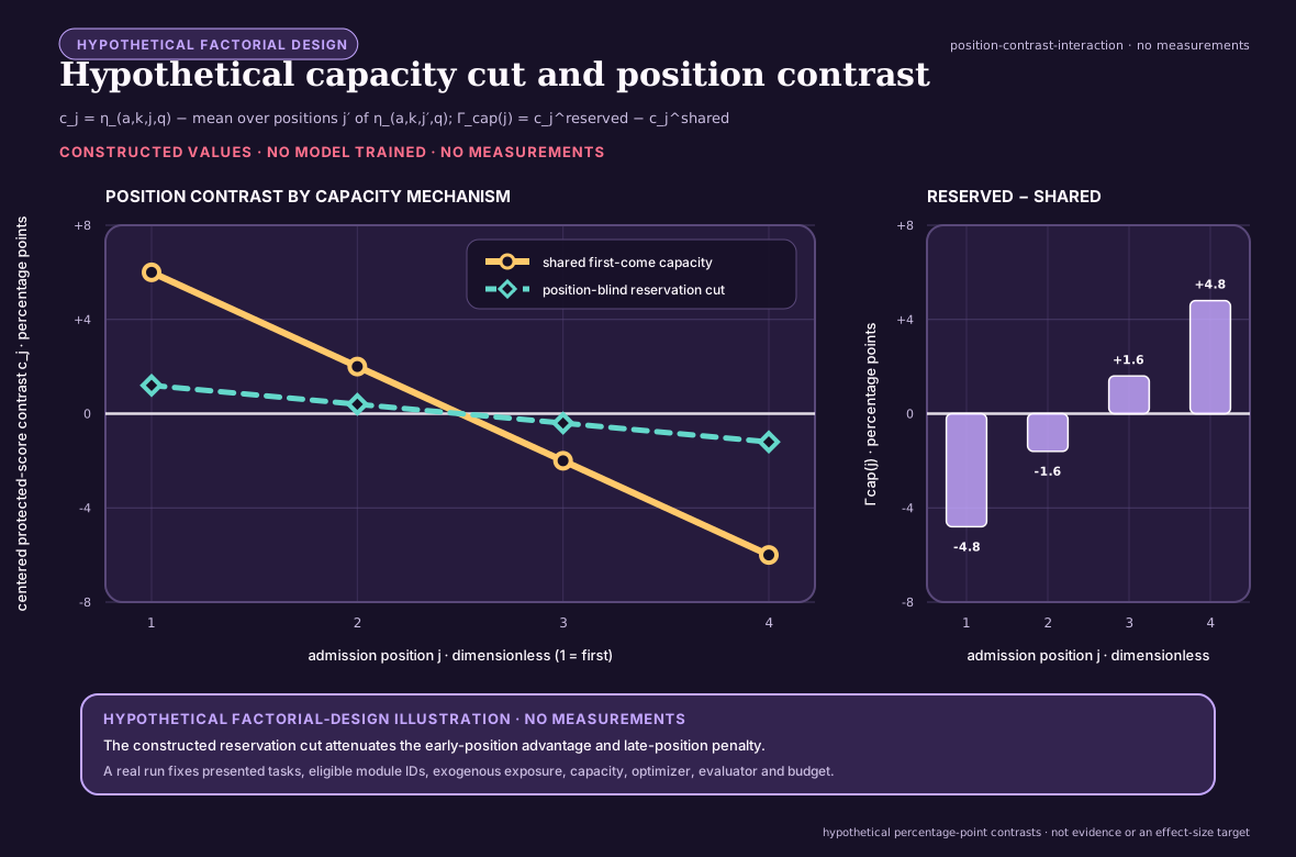
The history-conditioned modular-succession audit therefore reuses C-008, C-056, C-057, C-574, Fixture F-014, and Candidates 004 and 019 without creating another principle. Its residual test holds the task multiset, eligible module identity set, exogenous presentations, update ceilings, capacity, optimizer, evaluator and budget fixed, randomizes order, and separately cuts age, routed acceptance, capacity pre-emption, shared-state modification, facilitation and lock-in. If canonical replay, a non-learning scheduler, a mature continual-learning method, or a search-budget-charged curriculum explains the outcome, the biological transfer adds nothing.

New mechanisms can sharpen a principle without multiplying it

The developmental, regenerative, plant-plasticity, and multiscale-reduction depth passes add new failure boundaries without adding another universal principle. That is a useful result, not a failed search.

  • Positional memory and repair separate what state says should exist from which workers can currently rebuild it (C-1506, C-1507). They sharpen P-005, P-009, and P-012 by making write authority, reconstruction capacity, and current context separately testable.
  • Compensating sources, finite scaling, receiver geometry, delayed reinforcement, conditional redundancy, and local/global fields (C-1508C-1515) refine locality, maintenance, and structural offloading. They do not imply that every duplicated route, boundary, or organizer is useful.
  • Plant memory divides population-level digital switching, lifecycle reset, writing, trace maintenance, retrieval, systemic route identity, action-conditioned growth, and joint environmental context (C-1516C-1525). These are discriminating state and protocol dimensions inside P-002, P-005, P-006, P-009, P-012, and P-013—not a plant-themed architecture.
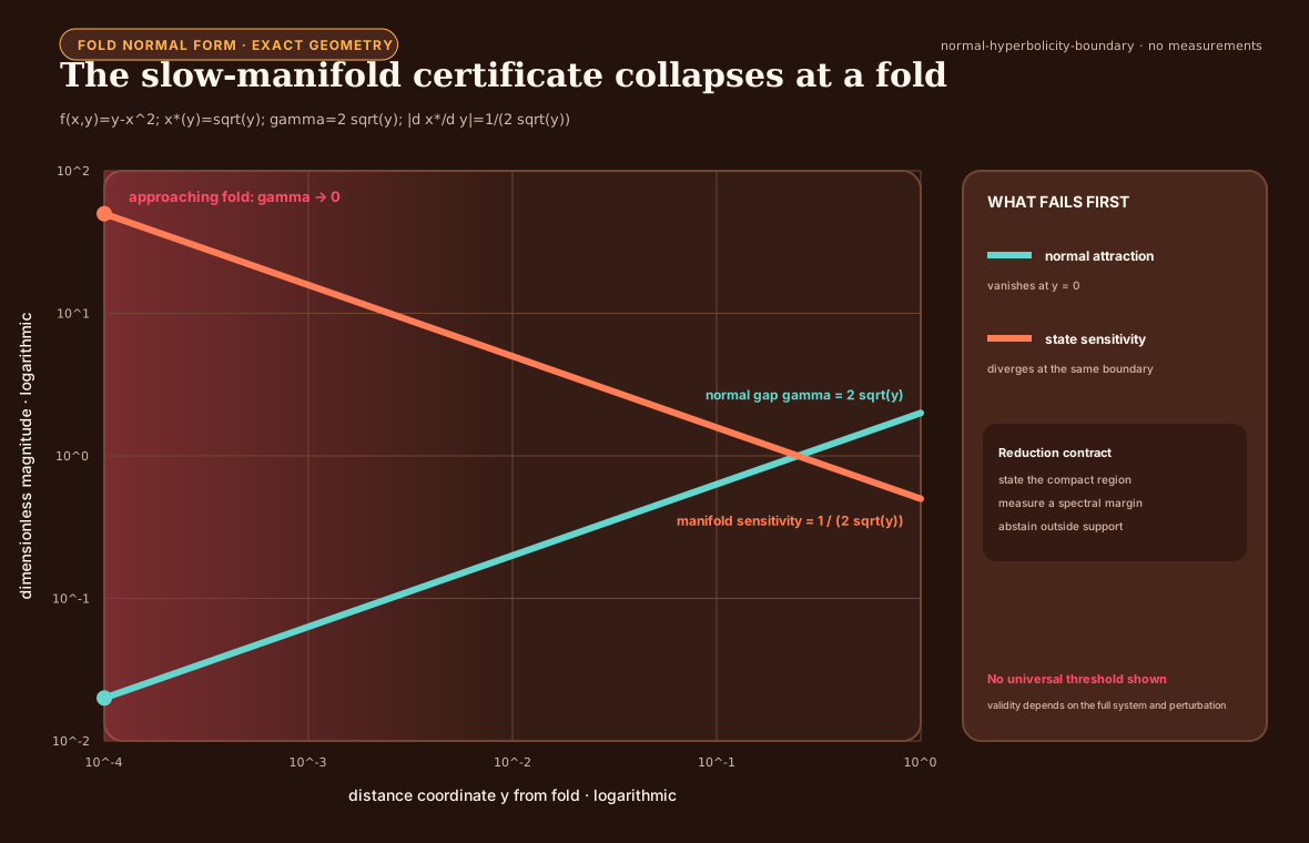
  • Projection memory, normal-hyperbolicity limits, macro-to-micro queries, and lift dependence (C-1526C-1529) supply mathematical rejection tests for coarse state. They constrain when an existing runtime or memory primitive is valid; they are not biological claims at all.

The deduplicated output is therefore richer in contracts while remaining at thirteen P-series principles. Fixtures F-022, F-023, and F-024 preserve the distinctions so later implementations can test whether a proposed composition adds value beyond its strongest ordinary null within a declared workload and transfer boundary.

Composition without double counting

Principles can cooperate while remaining separately testable. For one event:

  1. prediction-error allocation decides whether more evidence is valuable;
  2. selective allocation chooses a module within the active budget;
  3. local autonomy runs that module near its state;
  4. a temporary trace records unresolved credit;
  5. the maintenance plane later decides whether to replay, protect, merge, or forget it; and
  6. structural offloading compiles only the recurring path that survives those tests.

Calling the entire chain “sparsity,” “memory,” or “homeostasis” would hide which operation produced a gain. Each experiment therefore removes one principle at a time while holding the other interfaces constant.

Interconnection is an intervention

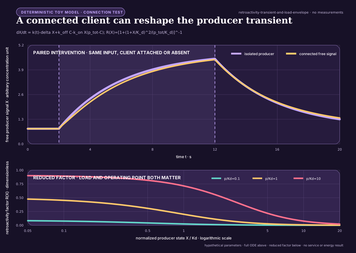
A small or typed interface does not by itself make two modules dynamically modular. In transcriptional regulation, covalent-modification cycles and yeast synthetic circuits, attaching a downstream target can alter the upstream state or transient response (C-1550C-1555). Substrate competition in Drosophila MAPK signalling supplies a distinct, potentially functional case (C-1559). The shared mechanism record is connection-induced back-action; the biochemical literature calls one important family retroactivity.

The domains do not collapse into one mechanism. Direct binding can sequester a signal, multiple substrates can compete for an enzyme, and nominally separate modules can instead couple through shared transcriptional, translational, CPU, memory, or scheduler resources (C-1558). The causal intervention therefore crosses connection state and shared-resource load independently. It also includes a genuinely nondestructive immutable-read control, because silicon can often copy or address state without the molecular consumption that motivated the analogy.

Insulation is bounded rather than automatically desirable. It must preserve both the producer and useful downstream service while exposing latency, staleness, copies, buffers, replicas, operations, maintenance and physical energy. Weak coupling may spend less while losing tracking or robustness (C-1556, C-1557); substrate competition can also be a useful integrator rather than a fault (C-1559). Fixture F-027 therefore compares suppressing, preserving and deliberately using back-action. If immutable messages, ordinary queues, resource isolation, explicit filters, stop-gradient paths or conventional controllers reach the same frontier, the translation is retired without adding a principle.

Passive self-organization is a mandatory null

Efficient-looking structure does not establish sensing, represented goals, or counterfactual action. Fracture sets, drainage networks, and river avulsions can arise from local stress, gravity, flow, conservation, thresholds, and stored geometry (C-232C-242). The project calls a mechanism adaptive control only when it specifies:

  1. a service variable external to the adaptation law;
  2. observations with spatial/temporal support and latency;
  3. a decision that could choose differently under different evidence;
  4. authority and an actuator;
  5. movement, reserve, monitoring, and recovery budgets;
  6. persistent state and reset cost; and
  7. a guarantee or tested failure envelope.

This criterion makes passive physics a stronger baseline. If local flow–structure feedback produces the same topology and service without a controller, the controller must justify its sensing, decision, switching, and maintenance cost. Connectivity is not throughput (C-234); material removed by “pruning” must appear as transport, storage, or output elsewhere (C-239); and a topology change can reassign or destroy service rather than improve it (C-242). A closed-form branching law is therefore a regime-qualified physical null, not a portable architecture rule (C-1489).

Transported fields are not messages

Microbial signals, metabolites, fungal nutrients, plant hormones, process streams, queues, and network packets can all create a local field that later receivers use. The common systems object is not “communication in nature.” It is a transported, transformed, delayed, and locally decoded quantity whose physical path may also change future capacity (C-563, C-578, C-580).

For transported type kk, use the local balance

ckt=Dk2ckuck+pkqkrkck,\frac{\partial c_k}{\partial t} =D_k\nabla^2c_k -\mathbf u\cdot\nabla c_k +p_k-q_k-r_kc_k,

where concentration ckc_k is mol/m³, diffusion coefficient DkD_k is m²/s, velocity u\mathbf u is m/s, production and uptake rates pk,qkp_k,q_k are mol/(m³ s), and first-order loss rkr_k is 1/s. Digital fields use an analogous typed byte or item ledger; they do not inherit molecular units or diffusion laws. Geometry, boundary conditions, sampling support, and receiver state are part of the contract. Countercurrent orientation is one finite exchanger arrangement inside that contract; it does not establish effectiveness or a generic bidirectional-computation benefit by itself (C-1490).

Several fields can be superposed at the same endpoints. If the observed outcome is

y=g=1Ghg(cg,θg)+b+ε,y=\sum_{g=1}^{G}h_g(c_g,\theta_g)+b+\varepsilon,

where GG is the number of typed channels, gg indexes one channel, cgc_g is its transported concentration or inventory, hgh_g is its receiver-dependent effect, θg\theta_g is channel state, bb is background, and ε\varepsilon is measurement error. Observing yy or cutting every channel together does not identify any one hgh_g. Each claimed channel needs an independently targetable intervention or a justified identification model. Rillig et al.'s concurrent-fungal-network perspective makes this problem explicit for fungal guilds sharing plant endpoints; the project adopts it as an engineering inference, not as evidence that such guild combinations have a demonstrated beneficial function (DOI, C-217, C-584).

flowchart LR
    P["Local production, release, or deficit"] --> T["Transport: flow · diffusion · delay · loss"]
    G["Geometry, topology, and boundaries"] --> T
    T --> C["Local concentration or typed inventory"]
    C --> R["Receiver state + uptake + response"]
    R --> O["Task outcome + local cost"]
    O --> U["Update source, sink, conductance, or topology"]
    U --> G
    C --> A["Accumulate · transform · consume · export · purge"]
    A --> C
    F["Damage, contamination, incompatibility"] --> X["Contain · isolate · reroute · regrow"]
    X --> G
    O --> V{"Independent validation"}
    V -->|"useful"| U
    V -->|"not useful"| D["Decay, disperse, or retire"]

Editable source: transported-field-contract.mmd.

The diagram deliberately spans several fields while retaining their differences:

  • microbial quorum output depends on production, confinement, flow, loss, and receptor state; it is not a vote count (C-563, C-575);
  • cross-feeding can help, harm, or create a weakest-link dependency, so local transfer is not system utility (C-571);
  • fungal flow can both deliver material and remodel conductance while rapid containment remains distinct from later bypass (C-577C-581); and
  • distinct symbiotic partners can exchange unequally under conflicting objectives (C-584); and
  • concurrent typed channels sharing endpoints remain causally unresolved when the experiment observes or disables only their aggregate.

The held fixture belongs jointly to P-011/P-013 and existing Candidates 001 and 013 (C-585). It must beat typed pub/sub or queues, fixed-graph adaptive routing, backpressure/primal–dual allocation, and make-before-break state transfer. Charge production, transport, storage, cleanup, contamination, topology edits, failed delivery, reserve, and measurement. If geometry and cleanup do not affect the task, use the simpler digital primitive.

Inactive is not one state

The immune evidence in C-727C-747 does not add another architecture principle. It contributes a stricter state contract. Representation, recognition, authentication, authorization, activation, suppression, deletion, impairment, contraction, memory, and recovery answer different questions and have different reversal costs.

flowchart LR
    G["Generate candidate rule / module"] --> R["Represent sampled evidence"]
    R --> V{"Developmental validation"}
    V -->|"insufficient coverage"| I["Ignorant · unresolved"]
    V -->|"unsafe with high support"| D["Delete + retain decision record"]
    V -->|"provisional pass"| N["Eligible but inactive"]
    N --> C["Context · provenance · current system state"]
    C --> A{"Recognition + authority + risk gate"}
    A -->|"permit"| X["Activate · expand · execute"]
    A -->|"monitor"| M["Observe without authority increase"]
    A -->|"quarantine"| Q["Anergic analogue · reversible disablement"]
    A -->|"external control"| S["Suppressed · rate-limited · scoped"]
    X --> O["Outcome · collateral loss · resource use"]
    O --> K["Contract · clean up · retain memory"]
    X -->|"persistent load or dysfunction"| H["Exhausted / impaired trajectory"]
    K --> P["Maintained memory · placement · expiry"]
    P -->|"qualified recurrence"| C
    I --> R
    M --> C
    Q -->|"revalidate"| C
    S -->|"authority changes"| C
    H -->|"diagnose + bounded intervention"| C
    O -->|"harm or false permit"| D

Editable source: typed-tolerance-lifecycle.mmd.

An activation bit cannot distinguish an absent module from an unobserved one, a policy-suppressed module from a damaged one, or post-response contraction from retained memory. That ambiguity makes reactivation unsafe and makes resource accounting wrong. Each transition therefore records evidence support, authority, expected useful effect, collateral-loss terms, resource budget, expiry, recovery target, and observed outcome.

Recognition supplies evidence; it does not grant authority. Deletion requires a higher support threshold than reversible monitoring or quarantine because a rare useful capability can be lost. Local copies pay maintenance, refresh, invalidation, and inconsistency costs. Recovery ends only when useful service and reserve are both restored.

The typed lifecycle mathematics compares this contract against a complete ordinary stack: typed state machines, calibrated risk and abstention, least privilege, constrained control, anomaly detection, evolutionary or ensemble search, replay, placement, and resource-aware scheduling. If the ordinary stack reproduces the decisions and frontier, the biological vocabulary is removed and the state contract remains.

Coordination without a privileged clock

Music cognition provides a combined stress regime for mechanisms that already exist elsewhere in the project: multiscale prediction, local timing control, transformation-aware memory, constrained generation, role protocols, repair, and cumulative transmission. The evidence in C-748C-783 does not justify a music-specific principle.

Its useful residue is a benchmark: agents must preserve literal phrase constraints and bounded relative timing while tempo, expressive microtiming, delay, roles, motifs, leaders, and partners change, without reading a privileged shared clock. Synchrony still requires common-input controls, edge interventions, and a protected functional endpoint before it can count as useful coordination (C-1495).

flowchart LR
    task["Score · cue · literal task constraints"] --> phrase["Phrase · motif · boundary state"]
    partner["Partner action"] --> channel["Delay · jitter · loss · acoustic/physical path"]
    channel --> observe["Timestamped local observation + uncertainty"]
    observe --> phase["Local phase · tempo · drift estimate"]
    memory["Partner · role · repertoire memory"] --> phrase
    phase --> controller["Role-qualified local controller"]
    phrase --> controller
    controller --> action["Timed expressive action"]
    action --> partner
    action --> evaluate["Literal task · synchrony · response · quality · cost"]
    evaluate --> repair["Correct · clarify · rehearse · update convention"]
    repair --> phrase
    repair --> memory
    nulls["PLL · Kalman · MPC · retrieval · typed protocol · rehearsal"] --> evaluate
    perturb["Tempo drift · role switch · leader loss · new motif · turnover"] --> channel
    perturb --> controller

Editable source: shared-clock-free-coadaptation.mmd.

The fixture refuses several easy substitutions:

  • similar mean tempo is not pairwise synchronization;
  • stimulus-frequency neural power is not evidence of endogenous prediction;
  • low onset error is not the correct phrase or role;
  • familiar-partner performance is not co-adaptation when retrieval explains it;
  • novelty is not validity, responsiveness, or usefulness; and
  • within-group convention compression is not cross-group task success.

Fixture F-001 compares the full composition with fixed correction, PLL/adaptive oscillator, Kalman identification, distributed MPC, a paid centralized conductor, transformation-aware retrieval, and typed role/version protocols. The mathematical contract keeps local clock error, phase, phrase prediction, role safety, message bytes, latency, rehearsal, recovery, and joules separate. If online estimation plus retrieval and explicit protocol state ties, the residual is retired.

Preserved bits are not preserved meaning

Library and archival science adds a dependency that storage abstractions often hide: information remains useful only for a declared interpreter community with the formats, schemas, vocabularies, identity mappings, authority evidence, software, units, permissions, and practiced capability needed to use it. The audit evidence will occupy C-784C-803.

flowchart LR
    object["Payload · metadata · evidence links"] --> package["Versioned preservation package"]
    community["Designated interpreter community + capabilities"] --> package
    dependencies["Format · schema · vocabulary · software · authority"] --> package
    queries["Registered queries · units · tolerances"] --> gate
    package --> transform["Retain · compact · migrate · emulate · delete"]
    transform --> candidate["Candidate version + manifest"]
    candidate --> gate{"Query · evidence · authenticity · access gates"}
    gate -->|"pass"| publish["Publish version + supersession lineage"]
    gate -->|"fail"| fallback["Retain source · narrow contract · repair"]
    publish --> drift["Community · dependency · vocabulary · authority drift"]
    drift --> invalidate["Invalidate · re-test · migrate · retire"]
    invalidate --> gate
    requests["New unregistered information need"] --> abstain["Answer if supported · otherwise abstain / recover source"]
    publish --> abstain
    outcomes["Task outcome · error · effort · cost"] --> queries
    publish --> outcomes

Editable source: query-registered-preservation.mmd.

This separates several failure modes that are otherwise mistaken for one success:

  • fixity detects bit change; it does not establish truth or authenticity;
  • provenance records lineage; it does not validate the assertion;
  • a valid ontology constrains representation; it does not prove instance data;
  • a citation edge is not endorsement or comparable impact;
  • findability and interoperability do not establish correctness or safe reuse; and
  • retaining records does not retain the tacit capability needed to interpret or act on them.

The query-registered preservation mathematics defines finite native-unit tolerances, evidence reachability, interpreter and dependency validity, migration regression, unregistered-query abstention, and complete lifecycle cost. The Candidate 017 track must beat ordinary OAIS/PREMIS-style packaging, versioned schema/vocabulary, retained-source recovery, and query-regression tests. If it does not, the ordinary preservation stack remains the implementation.

Candidate production is not acceptance

Mathematical practice supplies the sharpest version of a distinction already needed throughout this project: producing a candidate and earning acceptance are different operations. Conjectures, analogies, abstractions, proof sketches, retrieved lemmas, numerical patterns, solver traces, and learned tactic choices can all direct search. None of those origins establishes the resulting claim. The evidence and formal-system boundaries are tracked in C-861C-880.

The transferable lifecycle is typed:

  1. Propose. Bind a candidate to the exact problem, definitions, logic, axioms, library, corpus, proposal ancestry, and accessible evidence.
  2. Challenge. Search examples, counterexamples, countermodels, boundary cases, definition changes, and adversarial encodings before commitment.
  3. Decompose. Turn the target into a dependency DAG whose child artifacts reconstruct the parent goal through named interfaces and side conditions.
  4. Prove or refute. Produce a proof term, checked finite reduction, solver certificate, admissible model, or exact counterexample—not only a verdict.
  5. Check. Bind the artifact to the exact instance and library version, then run a small independent checker while publishing shared trust roots.
  6. Publish. Retain proved, refuted, tested, unknown, disputed, and retracted as different states with evidence, provenance, and cost.
  7. Invalidate. A definition, axiom, checker, dependency, or library change quarantines its reverse-dependency closure until rebuild or recheck.
flowchart LR
    identity["Immutable identity<br/>problem · definitions · logic · library · corpus · checker"] --> propose["PROPOSE<br/>conjecture · analogy · abstraction · candidate proof"]
    split["Dependency-safe split<br/>ancestor · sibling · restatement · source isolation"] --> propose
    propose --> challenge["CHALLENGE<br/>examples · countermodels · adversarial cases · critique"]
    challenge -->|"valid counterexample"| refuted["REFUTED<br/>typed counterexample + domain witness"]
    challenge -->|"survives finite tests"| tested["TESTED<br/>support range + precision + generator"]
    challenge --> revise["Revise statement · definition · abstraction"]
    revise --> propose
    challenge --> decompose["DECOMPOSE<br/>goal DAG · lemmas · interfaces · side conditions"]
    abstraction["Abstraction obligations<br/>soundness · adequacy · reconstruction · excluded cases"] --> decompose
    decompose --> prove["PROVE<br/>proof term · solver trace · model · exact finite reduction"]
    prove --> check["CHECK<br/>independent kernel or certificate checker"]
    separation["Generator/checker separation<br/>frozen input hash · explicit shared roots"] --> check
    check -->|"accepted certificate"| proved["PROVED<br/>scoped proposition + dependency closure"]
    check -->|"failed or unsupported"| unknown["UNKNOWN<br/>timeout · incomplete theory · malformed certificate"]
    refuted --> publish["PUBLISH<br/>versioned artifact · state · evidence · provenance · cost"]
    tested --> publish
    proved --> publish
    unknown --> publish
    disputed["DISPUTED<br/>formalization · assumptions · significance · review"] --> publish
    publish --> registry["Release registry<br/>proved · refuted · tested · unknown · disputed · retracted"]
    registry --> change["Dependency, definition, checker, or library change"]
    change --> invalidate["INVALIDATE<br/>reverse dependency closure · quarantine · recheck"]
    invalidate --> retracted["RETRACTED<br/>superseded state + reason + affected versions"]
    invalidate --> challenge
    nulls["ITP · ATP · CDCL · SMT · CP/MIP · CEGAR/CEGIS<br/>formal libraries · learned guidance · exact numerics · peer review"] --> compare{"Equal lifecycle budget<br/>hidden families · human-hours · joules"}
    registry --> compare
    compare --> retain["Retain measured residual<br/>otherwise retire composition"]

Editable source: versioned-proof-discovery-lifecycle.mmd.

This lifecycle prevents five common substitutions:

  • finite agreement is evidence for a tested range, not a universal result;
  • a counterexample rejects the encoded universal claim but does not choose its unique repair;
  • individually plausible lemmas do not close a parent goal unless their proof artifacts reconstruct it;
  • a checker establishes the encoded proposition relative to its logic, definitions, axioms, libraries, preprocessing, and trusted implementation; it does not validate the informal intent or importance; and
  • participant or model count does not establish independent checking when sources, parsers, libraries, prompts, or failure modes are shared.

Fixture F-004 compares the joined lifecycle with complete interactive and automated theorem provers, formal libraries, CDCL SAT, DPLL(T) SMT, constraint and model finding, CEGAR/CEGIS, learned premise/tactic guidance, exact numerical and exhaustive methods, and ordinary expert review. The mathematical contract defines immutable identities, leakage closures, abstraction obligations, proof-DAG reconstruction, certificate cost, typed states, invalidation, human effort, and joules. If the mature stack ties, the composition is retired; the state distinctions and negative result remain.

Efficiency mechanism

Deduplication saves two different resources.

First, it reduces research duplication. If plant priming, eligibility traces, and cache admission all motivate a temporary state before commitment, the project maintains one promotion interface and tests the domain-specific differences as variants. Papers and claims remain separate; architecture and instrumentation are reused.

Second, the resulting families define where the runtime should avoid repeated work:

  • scarcity families reduce unnecessary activation and acquisition;
  • locality families reduce movement and synchronization;
  • reversible-change families prevent every event from rewriting durable state;
  • maintenance families move repair and integration off the critical path; and
  • structural offloading reduces the recurring cost of mature behavior.

For principle jj, lifecycle acceptance uses the energy contract from chapter 80:

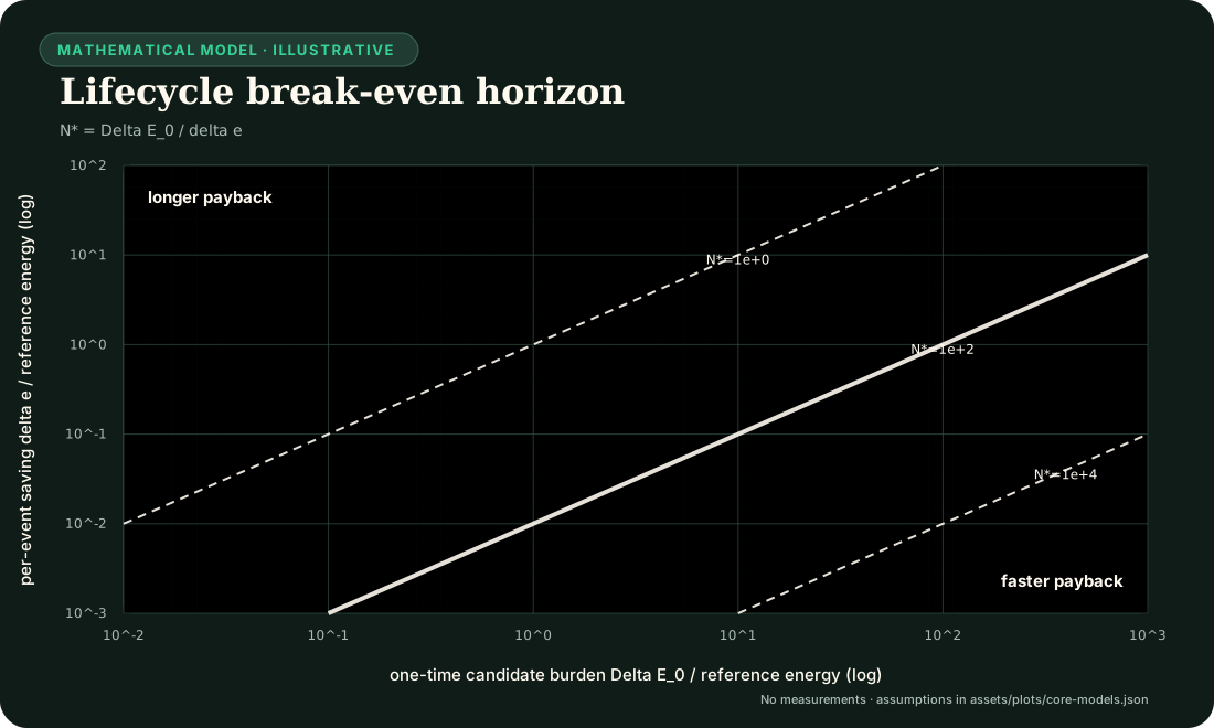
ΔEj(N)=N(EB,eventEj,event)Ej,introduceEj,maintainE[Ej,recover],\Delta E_j(N) = N\left(E_{B,\mathrm{event}}-E_{j,\mathrm{event}}\right) - E_{j,\mathrm{introduce}} - E_{j,\mathrm{maintain}} - \mathbb{E}[E_{j,\mathrm{recover}}],

where NN is a dimensionless count of qualified events, event terms are joules per qualified event, and introduction, maintenance, and expected recovery are joules over the same observation horizon. A positive ΔEj(N)\Delta E_j(N) is only an energy result; quality, risk, calibration, latency, and resilience must also remain inside their declared envelopes.

Evidence status

PropositionStatusBasis
several scientific domains expose recurring scarcity, locality, memory, stability, and structural pressuresestablished within the current scoped corpusclaims ledger and domain inventory
candidate production and scoped formal acceptance are different artifact statesestablished or plausible within the audited formal systems and experimentsC-861C-879; the joined lifecycle in C-880 remains plausible
the thirteen current principles are the correct deduplicationplausible working taxonomyprinciple registry; boundaries remain revisionable
five families provide a useful navigation layer without erasing mechanism differencesproposed synthesismust improve retrieval, experimental reuse, and reviewer agreement
recurrence across less-related domains predicts a useful artificial primitivespeculativerequires prospective tests against matched null models
the complete composition improves lifecycle efficiencyspeculativeisolated and composed experiments have not yet established it

Speculative extensions

  • Represent claims, principles, primitives, experiments, null models, and failures as a queryable versioned graph while keeping Markdown canonical.
  • Track negative results as first-class edges so a rejected translation is not repeatedly rediscovered under another domain name.
  • Estimate reviewer agreement on mechanism tuples before allowing a new principle ID.
  • Search specifically for counterexamples: fields where the same pressure produces a different stable solution or where the recurring solution fails.
  • Use contradictions between domains to generate new experiment regimes rather than averaging the difference away.
  • Maintain silicon-native escape routes beside every principle: exact copying, direct addressing, typed storage, rollback, high-speed communication, and variable precision can change which operation is cheapest.

Failure modes

  • Naming duplication: the same feedback loop appears repeatedly as a new organism-inspired component.
  • False convergence: similar diagrams hide different sensed variables, causal operations, or timescales.
  • Overcompression: a family becomes so broad that no ablation can isolate its mechanism.
  • Evidence laundering: recurrence is treated as proof of independence, optimality, or transfer to AI.
  • Null-model neglect: a familiar cache, scheduler, controller, or estimator is omitted because the biological story sounds novel.
  • Interface drift: two variants share a principle ID while receiving different inputs, budgets, or evaluation envelopes.
  • Positive-result bias: failed translations disappear, so the same proposal returns with a new metaphor.
  • Double-counted savings: two principles claim the same avoided operation or compare against different baselines.
  • Verifier laundering: checker acceptance is reported as truth about an informal statement without exposing formalization, axioms, dependencies, or the trusted implementation.
  • Finite-to-universal leakage: a sampled numerical or test range is silently promoted from tested to proved.
  • Correlated checking: producer and verifier share the parser, library, preprocessing, or defect that matters while being counted as independent.
  • Taxonomy lock-in: stable IDs are mistaken for immutable scientific truth.

Measurable predictions

  1. Independent reviewers given only normalized mechanism records agree on merge-versus-separate decisions more often than reviewers given titles and domain descriptions alone.
  2. As domain coverage grows, the number of supporting claims per accepted principle rises faster than the number of principles; a near one-to-one ratio signals failed deduplication.
  3. At least one proposed organism-specific mechanism is experimentally indistinguishable from an existing primitive at matched interface and cost and is removed rather than renamed.
  4. Experiments built around shared principles reuse telemetry, null models, and failure regimes across more than one source domain.
  5. Per-principle ablations attribute lifecycle savings to distinct avoided operations; overlapping savings disappear when all variants use one common baseline and boundary.
  6. A principle promoted from recurrent evidence survives at least one regime derived from a domain outside the one that originally motivated its AI translation.
  7. A typed propose–challenge–prove–check lifecycle reduces bad acceptance, localizes repair, and improves dependency invalidation beyond a generator plus checker alone after search, certificates, libraries, human effort, and joules are charged; otherwise Fixture F-004 retires the composition.

Concept · 4,412 words

Structural growth, specialization, and conditional routing

Scope

Define how a modular system acquires new capacity without running, training, or retaining every possible module for every event. Growth is admitted only for a measured capability gap, new capacity earns traffic in probation, and mature capacity remains eligible for merge, reopening, or retirement.

The central object is a capacity lifecycle, not a continuously expanding pool. Birth, routing, specialization, placement, consolidation, and removal are separate decisions with separate costs.

Biological observation

Developing nervous systems generate and reorganize more cells and connections than remain in mature circuits. In the studied mouse retinogeniculate system, relative activity and complement signaling changed microglial engulfment and retention of developing inputs (C-043). This supports activity-sensitive structural refinement by a slower maintenance process, without specifying one general pruning rule.

Protection is not necessarily permanent. Targeted extracellular and receptor interventions reopened specific forms of adult visual-cortex plasticity (C-044, C-045). The resulting engineering states are candidate, consolidating, protected, reopened, and retiring. A module can be stable without becoming impossible to revise.

Other biological systems expose control operations that recur at different scales:

  • germinal-center affinity maturation combines variation, selection, expansion, and later protection of useful lineages (C-028);
  • Physarum and fungal networks couple use-dependent reinforcement, exploration, fusion, and contraction to changing flow (C-027, C-034);
  • ants can open reserve routes under crowding before throughput falls (C-035); and
  • activity can recruit local energy production, alter resource placement, and change local vascular supply in scoped neural preparations (C-049C-051).

These mechanisms are not interchangeable. Together they impose a useful system constraint: variation and reserve capacity consume resources; selection needs an independent test; frequently used structure may stabilize; unused or duplicated structure must be able to leave the hot path.

A defined microbial-community experiment adds a practical design tactic: adding candidates selected for missing functions repaired the tested community better than merely restoring organism count (C-056). The inverse problem also matters. Functional redundancy was associated with poor newcomer engraftment in two small reanalyzed human microbiome datasets (C-057). Mature capacity can resist both harmful and beneficial entrants, so an artificial newcomer needs protected evaluation traffic rather than permission from incumbent routing logits alone.

Proposed AI translation

The capacity lifecycle

flowchart LR
    subgraph birth["1 · Detect and birth"]
        direction TB
        gap["Persistent capability gap"] --> proposal["Clone · seed · compose"]
        proposal --> probation["Probation<br/>bounded state + budget"]
    end
    subgraph compete["2 · Route and specialize"]
        direction TB
        trial["Exploit · explore · reserve traffic"] --> evidence{"Useful, distinct,<br/>and affordable?"}
        evidence -->|"yes"| specialize["Local specialization"]
        evidence -->|"no value"| discard["Discard + retain result"]
        evidence -->|"duplicate"| merge["Merge or distill"]
    end
    subgraph lifecycle["3 · Consolidate or release"]
        direction TB
        gate["Maturity gate"] --> protected["Protected module"]
        protected --> monitor["Quality · traffic · cost · fragility"]
        monitor -->|"redundant"| retire["Drain + retire"]
    end
    probation --> trial
    specialize --> gate
    merge --> gate
    monitor -->|"new gap"| gap
    retire --> released["Released hot capacity"]

Editable source: ../assets/diagrams/structural-growth-routing.mmd.

The initial system contains modality encoders, predictive shared state, conditionally addressable experts, hierarchical routers, episodic and factual memory interfaces, and a declared reserve. Total addressable capacity may be large, but each event receives only a bounded route. Reserve capacity is stored, placed, and periodically tested; it is not free merely because it is inactive.

1. Detect a capability gap

Growth begins with a gap record, not a global loss spike. A valid record groups attributable episodes that existing routes fail in a consistent way and asks whether the failure is better explained by:

  • missing capability;
  • insufficient active compute or depth;
  • missing context or memory;
  • router error or capacity congestion;
  • interference inside an existing module;
  • distribution drift; or
  • corrupted data, tools, or feedback.

The maintenance plane attempts the cheaper explanations first. New capacity is eligible only when the gap persists across resampling or recurrence, existing modules cannot absorb it inside their interference and resource bounds, and a candidate has a declared validation contract. This ordering prevents every hard example from becoming an expert.

2. Choose a birth operation

The proposal names both the new structure and what it is expected to repair:

Birth operationBest initial conditionPrincipal cost
Clone and divergeone incumbent is close but suffers interferencecopied parameters, optimizer state, later deduplication
Activate a seedthe gap is genuinely outside active coveragestored reserve, cold-start training, placement
Compose a moduleexisting primitives are adequate but repeatedly coordinatedrouter depth, boundary traffic, compilation work
Reopen a protected modulea previously valid skill must changeregression risk, branch validation, rollback

Every birth creates a versioned provisional module. It cannot write the slow model, replace an incumbent, or claim permanent memory during probation. Initialization source, training episodes, expected role, resource ceiling, and discard path are recorded before it receives traffic.

Composing or admitting that module is itself a perturbation. The newcomer can pin shared activations, add router or queue pressure, alter normalization, create a gradient path, mutate shared cache state, or intentionally feed back. Before probation credit is assigned, compare the incumbent producer under the same input and seed with the connection absent and present. Cross connection state independently from shared CPU, memory and scheduler load so ordinary contention is not mislabeled as connection-induced back-action (C-1550, C-1558). Immutable snapshots, bounded queues, resource isolation, stop-gradient adapters and explicit feedback remain the minimum nulls. The full qualification and retirement rules are in Fixture F-027.

Birth order is another intervention, not a background detail. A newcomer that arrives first can be older, receive more examples, pre-empt finite capacity, modify shared state, facilitate a later module, or create a costly lock-in. Those mechanisms predict different remedies. The same task multiset and eligible module identity set must therefore be replayed across randomized orders with equal exogenous presentations, task-local update ceilings, capacity, optimizer, evaluator and lifecycle budgets. Realized active, consolidated, merged, or retired state remains an outcome. Routed acceptance remains a measured mediator and is equalized only in the exposure-cut cells. Canonical replay, ordinary scheduling, replay/EWC/OGD, fixed and capacity-matched MoE, random curricula, optimized curricula with their search cost, population-based training and quality-diversity search are the required null stack. The exact factorial and kill rules are in the history-conditioned succession contract.

3. Give the candidate probation traffic

The router divides admitted work into three explicit budgets:

  • exploit traffic goes to the strongest validated route;
  • exploration traffic compares plausible candidates on informative events; and
  • reserve traffic preserves failover and tests paths that would otherwise decay unnoticed.

A newcomer receives a capped share of gap-relevant episodes plus matched control episodes. The control traffic reveals whether it learned a capability or merely a narrow identifier for the failure cluster. Incumbents cannot reduce the evaluation share through their own confidence, but the maintenance plane can stop the trial for quality, risk, latency, memory, or energy violations.

For event xx, use a dimensionless routing objective

Lroute(x)=Ltask(x)+λEE^(x)E0+λBB^(x)B0+λbalLbalance(x)+λchurnLchurn(x),\mathcal{L}_{\mathrm{route}}(x) = \mathcal{L}_{\mathrm{task}}(x) + \lambda_E\frac{\widehat E(x)}{E_0} + \lambda_B\frac{\widehat B(x)}{B_0} + \lambda_{\mathrm{bal}}\mathcal{L}_{\mathrm{balance}}(x) + \lambda_{\mathrm{churn}}\mathcal{L}_{\mathrm{churn}}(x),

where E^(x)\widehat E(x) is estimated joules/event, B^(x)\widehat B(x) is estimated bytes/event across named memory and network boundaries, and E0E_0 and B0B_0 are declared reference scales with the same units. All λ\lambda coefficients and losses are dimensionless. The physical joule and byte measurements remain separate reported outcomes; normalization does not turn them into task quality.

Balance keeps one expert from taking all traffic. Churn is applied only after a route has accumulated evidence of stable specialization; penalizing early movement would protect arbitrary initialization.

When module reports become strategic

Ordinary routing remains the default. Shadow-price feedback already represents scarcity under declared controller conditions (C-133), and auction or matching language adds nothing when the router can observe costs and every module shares the system objective. A market-like mechanism is in scope only when a persistent module holds decision-relevant private information, can improve its future traffic by misreporting, and faces a real opportunity consequence it cannot reset or evade.

That regime creates specific failures. Selection pressure on a visible metric can damage poorly measured substitute tasks (C-139); proper scoring needs an independently verified outcome and does not establish competence or causal contribution (C-140); peer agreement can reward shared error or collusion (C-141); and fixed-agent truthfulness does not solve false identities or a biased allocator (C-143).

Candidate 008 therefore begins with a cooperative applicability control that it should not beat. Only then does it introduce hidden costs, adaptive metric gaming, protected outcomes, entrants, identity resets, collusion, and allocator deviation. Withheld audits, lineage-bound consequences, protected entrant traffic, and replayable commitments remain only if they improve external task, risk, energy, and latency outcomes after their evaluation and storage costs.

4. Measure specialization rather than naming it

A candidate becomes useful when it improves a defined region of behavior while remaining distinguishable from existing modules. Evidence includes:

  • causal improvement when the candidate is admitted and regression when it is ablated;
  • reduced interference on incumbents or protected history;
  • consistent advantage on held-out gap and recurrence episodes;
  • a stable but non-exclusive routing region;
  • calibration and rare-case behavior inside its declared envelope; and
  • physical cost that remains inside its allocation.

Low routing entropy alone is not specialization: a router can collapse onto a module for the wrong reason. High activation diversity alone is not useful: a pool can fragment one capability across many expensive duplicates. The test is complementary causal contribution at a measured lifecycle cost.

5. Hand off to merge, protection, or retirement

At the end of probation, the candidate has three normal outcomes:

  1. Discard. It adds no reliable capability. Preserve the negative result so the same proposal is not regenerated indefinitely.
  2. Merge or distill. It reproduces an incumbent or several modules have converged on one operation. Build a compact branch, rerun intervention and recurrence tests, then drain duplicates.
  3. Consolidate. It contributes a distinct reusable capability. Pass it to the maturity lifecycle for protection, reopening rules, structured pruning, and rollback.

A protected module remains monitored for traffic, unique contribution, physical placement, recovery, and newcomer exclusion. Persistent redundancy returns it to a merge-or-retire gate. Logical topology changes can be evaluated with Candidate 001, which charges reconfiguration, migration, reserve, controller, and recovery costs.

Conventional null models

The growth controller must beat ordinary ways of allocating or restructuring capacity, not only a frozen weak model:

IDNull modelWhat it tests
N0Capacity-matched dense monolithwhether modular growth is needed at all
N1Fixed-capacity sparse MoE with tuned load balancingwhether conditional routing alone explains the gain
N2Fixed modules plus adapters or low-rank updateswhether new structure beats ordinary parameter-efficient adaptation
N3Periodic global architecture or topology optimizationwhether a standard batch redesign explains local lifecycle control
N4Usage- or magnitude-prune/retrain cyclewhether causal merge/retire gates add value
N5Random valid birth, merge, and retirement under equal budgetswhether the lifecycle signals carry information
N6Trace-aware oracle with future gap labelsunattainable ceiling; never a superiority baseline

Equalize initial capacity, maximum stored capacity, active work, optimizer updates, training examples, router information, tuning trials, migration bytes, validation work, and wall-clock opportunity. Charge candidate failures and discarded births. Otherwise growth buys more search while the null models are asked to solve the task in place. A stylized optimum such as a fixed branching exponent belongs in this null stack only inside its verified objective, transport law, and constraint regime (C-1489).

A topology change carries state

Changing an edge label is not the same as transferring a working system. The process-engineering audit makes the missing state visible: an installed path may hold inventory, energy, contamination, pending work, actuator authority, wear, calibration, maintenance obligations, and shared protection dependencies (C-501, C-510). Two endpoint configurations can both be feasible while the path between them is unsafe (C-512). Static branching relations do not remove that transition state (C-1489); fast allocation and slow structural adaptation must retain separate action, deficit, build, stranded-capacity, and recovery histories (C-1496).

For digital modules, use a typed transition inventory rather than pretending that bytes obey material conservation. For state class kk,

Ik(t1)Ik(t0)=AkDkXk+Rk,I_k(t_1)-I_k(t_0) = A_k-D_k-X_k+R_k,

where IkI_k is bytes present at a named boundary, AkA_k is admitted bytes, DkD_k is deliberately deleted bytes, XkX_k is exported bytes, and RkR_k is internally replicated bytes over [t0,t1][t_0,t_1]. Each term is bytes and carries a provenance, validity, and ownership version. This is an accounting contract, not a claim that information is physically conserved (C-517).

flowchart LR
    P["Proposed graph version"] --> G{"State, cost, and safety gate"}
    I["Queued · cached · provisional state"] --> G
    A["Authority · dependencies · fallback"] --> G
    G -->|"admit"| T["Shadow and bounded transfer"]
    G -->|"reject"| K["Keep fixed graph"]
    T --> V{"Observed postcondition"}
    V -->|"pass"| N["New active version"]
    V -->|"fail"| R["Drain and roll back"]

Editable source: conservation-qualified-reconfiguration.mmd.

Candidate 001 therefore includes a physical stress track. It must beat fixed-graph adaptive control, multi-mode supervisory control, and offline redesign after installed reserve, transition state, flushing, downtime, maintenance, and rollback are charged. If those nulls tie it, “adaptive topology” describes an implementation choice rather than an efficiency mechanism (C-516).

Positional instruction, repair capacity, and structural fields

The developmental and regeneration residue sharpens the capacity lifecycle by separating operations that a generic “grow and repair” controller would hide. The claims are source-domain results; their engineering translations remain prospective and are tested only by the preimplementation F-022 fixture.

  1. Keep repair instruction distinct from repair workforce. In the studied planarian experiments, differentiated muscle carried position-control expression while neoblasts supplied replacement capacity (C-1507). A modular system should therefore test a two-plane design: surviving task modules retain bounded reconstruction constraints, while a replaceable worker pool executes them. A worker reserve is not positional knowledge, and retained instructions are not proof that enough capacity survives. DEV-T02 compares this separation with complete checkpoint-and-log restoration and requires abstention when surviving instruction support is insufficient.
  2. Treat positional memory as writable, gated state. Transient intervention rewrote persistent positional state during the scoped axolotl regeneration window, but not in comparable uninjured cells (C-1506). The translation is neither immutable metadata nor unrestricted self-editing: retain versioned local role state, open writes only inside an authenticated repair episode, validate against independent service evidence, and preserve rollback. DEV-T01 makes valid, locally corrupted, and common-mode-corrupted memory separate cases so saved reconstruction work cannot excuse confident wrong-role repair.
  3. Separate source compensation, scale support, and receiver observability. Opposed BMP-related sources compensated for scoped perturbations in Xenopus (C-1508); DEV-T03 asks whether reciprocal sources beat distributed robust control after delay, stability, and double-source detection are charged. Dpp-gradient scaling in the studied wing disc had an experimentally exposed finite envelope (C-1509); DEV-T04 therefore requires an explicit beyond-support disposition rather than a scale-invariance claim. In the cited micropattern assay, edge access and receptor orientation changed which signal a cell could observe (C-1510); DEV-T05 compares local boundary-relative inference with exact distributed graph distance. A compensating field can still be unreadable at the receiver, and a readable field can still be outside its calibrated size range.
  4. Consolidate paths and boundaries only after persistent evidence. Tension recruited and stabilized Myosin II in the scoped tissue experiments (C-1511), motivating capped, decaying load-path reinforcement rather than permanent reinforcement after a burst; DEV-T06 includes load reversal and event-triggered backpressure as controls. An actively maintained Myosin-II barrier limited compartment mixing (C-1512), motivating delayed, reversible interface hardening tested against a mature soft boundary in DEV-T07. Apparent enhancer redundancy improved robustness only across particular perturbations in the studied loci (C-1513); DEV-T08 accordingly tests partially input-diverse small gates against full duplicate controllers and preserves common-mode corruption as a hostile null.
  5. Compose local patterning with coarse global context without conflating their roles. The limb-pattern study supports a plausible, non-unique reaction–diffusion interpretation modulated by global gradients (C-1514). DEV-T09 therefore requires local-only and global-only ablations and compares the composition with central constrained assignment. Chick perturbations also support local-feedback symmetry breaking, while the proposed molecular model remains non-unique (C-1515); DEV-T10 tests temporary organizer election against a complete randomized leader-election protocol, including duplicate detection and re-election.

These distinctions add three gates to structural growth: verify that surviving instruction is sufficient before allocating repair workers; verify that the field is both inside its support envelope and observable by the receiving module; and verify that reinforcement or boundary writes amortize their write, maintenance, reopening, and fallback costs. Every F-022 track remains NO_RESULT; a written protocol does not establish an efficiency advantage.

Competence-gated structural transition

A signal is not a complete command. Developmental experiments show that concentration, duration, position, stage, and receiver state can change the response to the same extracellular input (C-539C-549). Commitment can later be redirected, but reopening is an intervention with selection, resource, integrity, and safety costs rather than free reversal (C-550, C-551).

For module mm and transition-contract version vv, define the dimensionless admission predicate

Gm,v(t)=1 ⁣[qm(t)Cv,tWv,em(t)θv,rm(t)rvmin,Rm,v(t)=1].G_{m,v}(t)= \mathbf 1\!\left[ q_m(t)\in\mathcal C_v, t\in W_v, e_m(t)\ge\theta_v, \mathbf r_m(t)\succeq\mathbf r_v^{\min}, R_{m,v}(t)=1 \right].

qm(t)q_m(t) is typed local competence state; Cv\mathcal C_v is the permitted state region; tt is seconds; WvW_v is a declared time interval in seconds; eme_m and evidence threshold θv\theta_v are dimensionless; resource vectors rm\mathbf r_m and rvmin\mathbf r_v^{\min} are compared componentwise in their native units; and Rm,vR_{m,v} is a dimensionless predicate that a tested rollback path exists. The signal is eligible to create a provisional transition only when Gm,v=1G_{m,v}=1.

stateDiagram-v2
    [*] --> Incompetent
    Incompetent --> Eligible: local state enters window
    Eligible --> Provisional: signal + evidence + resources
    Provisional --> Committed: validation passes
    Provisional --> Incompetent: reject + reset
    Committed --> Protected: structural postcondition
    Protected --> Reopening: explicit trigger + budget + rollback
    Reopening --> Provisional: bounded retrial
    Reopening --> Protected: abort + restore
    Protected --> Retiring: replacement or lost utility
    Retiring --> [*]: drain + retain evidence

Editable source: competence-gated-transition.mmd.

The fixture splits responsibilities instead of adding another candidate:

  • Candidate 002 tests low-bandwidth signal decoding by versioned receivers;
  • Candidate 009 owns admissibility, authority, dependencies, and invalidation;
  • Candidate 010 owns provisional evidence before commitment and reset;
  • Candidate 006 owns structural write, health, shadow, and physical reopening; and
  • Candidate 014 owns support, stage, vintage, and the observations defining competence.

Reject the composition if an ordinary gate, schedule, staged verifier, and versioned migration procedure matches quality, interference, rollback, availability, bytes, latency, and joules. The fixture is useful only if the interaction among signal, receiver history, finite window, commitment, and reopening predicts failures those separate controls miss (C-562).

When the unit of adaptation changes

A cooperating set of modules is not automatically a higher-level unit. The claim becomes testable only after defining its boundary, child-configuration event, inherited state, within-lifetime state, descendant relation, collective performance, member-level incentives, and conflict-control cost. This separates aggregation from individuality and a demographic bottleneck from a reproducible founder boundary (C-282C-295).

flowchart LR
    F["Versioned founder / propagule"] --> C["Reproducible collective configuration"]
    C --> V["Bounded within-lifetime variation + specialization"]
    V --> T["Collective task outcome"]
    T --> P["Partition collective gain vs member shortcuts"]
    P --> G{"Joint gain survives conflict cost?"}
    G -->|"no"| X["Use ordinary modular control"]
    G -->|"yes"| H["Select reproducible higher-level lineage"]
    H --> F
    V --> A["Audit · budget · sanction · reproductive separation"]
    A --> P

Editable source: conflict-bounded-unit-transition.mmd.

For collective lineage kk, let ZkZ_k be task-native collective performance and WkW_k its dimensionless admitted-descendant weight. The selection accounting is

ΔZˉ=Cov(Wk,Zk)Wˉ+E[WkΔZk]Wˉ.\Delta\bar Z= \frac{\operatorname{Cov}(W_k,Z_k)}{\bar W} +\frac{\mathbb E[W_k\Delta Z_k]}{\bar W}.

The first term is change among declared collectives and the second is transmission change. A nested partition separately reports member-level shortcuts. The identity is accounting, not causal proof; group and descendant definitions are preregistered. Candidate 016 must beat typed modular systems, permissions and tests, clean versioning, external evaluation, routed experts, and ensemble/population selection after enforcement, false-sanction, interface, founder, reserve, and recovery costs.

Efficiency mechanism

For experts i=1ni=1\ldots n, let gi(x){0,1}g_i(x)\in\{0,1\} be the dimensionless event gate, Ci(x)C_i(x) be executed operations/event under a declared precision, and Crouter(x)C_{\mathrm{router}}(x) use the same convention:

Cactive(x)=Crouter(x)+i=1ngi(x)Ci(x).C_{\mathrm{active}}(x) =C_{\mathrm{router}}(x)+\sum_{i=1}^{n}g_i(x)C_i(x).

This separates addressable parameter capacity from executed work, as sparse mixture-of-experts systems demonstrate in specific implementations (C-003). It does not price parameter reads, dispatch, all-to-all communication, imbalance, cold starts, or maintenance.

The lifecycle energy per served event is therefore

Eˉcapacity=Eroute+i=1ngiEi+Ecomm+Ebirth+Etrain+Eplace+Evalidate+Emerge/retire+E[Erecovery]Nserved,\bar E_{\mathrm{capacity}} = E_{\mathrm{route}}+\sum_{i=1}^{n}g_iE_i+E_{\mathrm{comm}} +\frac{ E_{\mathrm{birth}}+E_{\mathrm{train}}+E_{\mathrm{place}} +E_{\mathrm{validate}}+E_{\mathrm{merge/retire}} +\mathbb{E}[E_{\mathrm{recovery}}] }{N_{\mathrm{served}}},

where every EE term is in joules, EiE_i is expert execution energy/event, and NservedN_{\mathrm{served}} is the number of events over the comparison horizon. Report stored parameter and optimizer bytes, bytes moved/event, latency, utilization, quality, calibration, and risk alongside energy.

Growth is efficient only if conditional execution saves more than candidate search, idle reserve, placement, validation, and later contraction consume. Lottery-ticket results show that competitive sparse subnetworks can exist in tested settings (C-012); they do not establish that this lifecycle discovers them or realizes energy savings on a target system.

Evidence status

ElementStatusRole in this chapter
conditional expert routing (C-003)established in published systemscapacity and active compute can be separated in suitable implementations
competitive sparse subnetworks (C-012)established in tested settingsstaged selection and pruning are viable operators
use-dependent biological topology (C-027, C-034)established in scoped organisms/modelsmotivates reinforcement, decay, exploration, and contraction tests
diversity, selection, and protection (C-028)established in the cited immune experiment/modelmotivates a bounded candidate lifecycle
congestion-triggered reserve use (C-035)established in the cited ant setup/modelreserve paths should be priced and tested before overload
developmental refinement and reopening (C-043C-045)established in scoped neural preparationssupports distinct candidate, protected, and reopened states
local resource demand and placement (C-049C-051)established in scoped neural preparationsphysical supply and movement belong in routing cost
shadow prices, matching, proper scoring, metric pressure, identity, and allocator credibility (C-133C-143)established under scoped economic models and experimentsordinary routing remains the null; contestable allocation is conditional on a measured strategic-information problem
audit-backed contestable allocation (C-144)speculative systems compositionCandidate 008 must lose its distinction when modules are cooperative and directly observable
capability-gap repair (C-056)established for the defined mouse community and challengemotivates selecting additions by missing function
functional redundancy and engraftment (C-057)plausible associationmotivates protected newcomer evaluation and a lock-in test
higher-level heredity and conflict accounting (C-282C-295)scoped population-genetic and evolutionary results; artificial composition speculativeCandidate 016 tests whether a collective becomes a useful adaptation unit beyond ordinary modular lifecycle controls
complete grow–route–specialize lifecyclespeculative synthesisrequires comparison with N0–N6

Speculative extensions

  • Let modules request a birth trial with a compact capability-gap certificate; maintenance allocates the trial, not the requesting module.
  • Maintain seed modules at several parameter and precision scales so a new role need not start from the largest available structure.
  • Learn placement jointly with specialization only after migration cost and rollback are measurable.
  • Use recurrence-aware cold storage: retire a module from hot execution while retaining enough checkpoint and routing evidence to restore it if its regime returns.
  • Allow two candidates to share an encoder or memory interface while keeping their update authority and resource accounts separate.
  • Test local birth/retirement against periodic global architecture optimization under recurrent rather than one-way task sequences.

Failure modes

FailureObservable signatureRequired response or ablation
Router collapseone module takes most traffic; queue tails or overflow risefixed-capacity MoE and stronger load-balancing baseline
Candidate inflationbirth rate and stored bytes rise without held-out gap closurecap trials; compare no-growth and random-birth nulls
Fragmentationmany modules show overlapping ablation effects and high boundary trafficmerge/distill branch with causal coverage tests
Incumbent lock-ina superior newcomer cannot acquire evaluation trafficreserved probation share; compare router-logit admission
Premature localizationmodality-specific routes lose cross-modal transfershared-module and monolithic controls on compositional tests
Reserve starvationno path remains for faults or new regimesprice and enforce declared reserve capacity
Reconfiguration thrashrepeated births, moves, merges, or retirements dominate costhysteresis and slower maintenance epochs
Stranded capacitycold modules occupy memory but never serve, fail over, or restorecold-storage, deletion, and restore-value comparison
Cosmetic sparsityactive gates fall while loaded bytes, communication, or joules do nothardware trace and dense-kernel ablation
Maintenance inversionsearch, validation, migration, and rollback cost exceeds runtime savingfull lifecycle equation and fixed-structure nulls
Rare-role deletionaverage quality holds while rare or safety-critical cases regressprotected recurrence suite and reconstructable checkpoint
False higher-level unitaggregate reward rises but collective inheritance is transient or member shortcuts dominatepreregister descendant relation; selection partition; ordinary modular and external-evaluator nulls

Measurable predictions

  1. Capability-gap-driven births close held-out failure clusters with fewer admitted candidates and lower lifecycle energy than random birth, periodic fixed growth, and capacity-matched adapter baselines.
  2. A protected probation share lets genuinely better newcomers establish causal value faster than incumbent-logit admission without increasing harmful promotions at the same validation budget.
  3. Successful specialization produces a stable, non-exclusive routing region and positive unique ablation value; routing entropy alone predicts promotion less reliably.
  4. Conditional growth reduces executed operations and bytes moved/event relative to a capacity-matched monolith while preserving quality, calibration, and rare-case performance.
  5. Causal merge/retire gates preserve recurring and intervention capability better than usage- or magnitude-only pruning at matched hot capacity.
  6. Reserve capacity improves recovery after faults or returning regimes enough to justify its stored bytes, idle energy, and periodic test traffic.
  7. Joint routing and placement lowers communication energy only after migration, cold-start, and rollback work are included.
  8. A collective lifecycle advances only when cost-adjusted between-collective selection and inherited capability persist under member shortcuts and turnover beyond ordinary lifecycle governance.
  9. The complete lifecycle advances only if it improves the quality–risk–latency– energy–adaptability frontier over N0–N5; a parameter-count or FLOP reduction alone does not satisfy the prediction.

Concept · 5,999 words

Multimodal sensorimotor grounding

Scope

Grounding means that a model’s state is constrained by temporally ordered observation, action, and consequence—not that every concept must be reducible to pixels or motor commands. This chapter defines the trajectory record from which such state can be learned, how language attaches to it, and the tests that separate action-conditioned structure from passive multimodal correlation.

The central unit is a versioned episode containing asynchronous sensor events, commanded and realized interventions, exogenous events, and language with provenance. The model must predict and act under missing modalities, timing error, partial observability, and finite sensing energy. A representation is treated as grounded only to the extent that it supports held-out prediction, intervention, control, and reference at a declared uncertainty.

Biological observation

Biological perception is embedded in a closed loop. During active whisker exploration, measured contact mechanics predicted primary sensory-neuron firing better than whisker angle alone in the scoped mouse experiment (C-022). The result establishes that self-generated sensing mechanics can matter to the sensory code; it does not make embodiment necessary for every capability.

Other evidence constrains parts of the translation:

  • sparse coding can learn localized structure from natural images in the model studied under C-002;
  • latent target prediction can learn semantic image representations without pixel reconstruction under C-006;
  • children in a controlled toy study targeted actions toward unresolved causal structure under C-062;
  • pedagogical demonstration narrowed subsequent exploration in the scoped toy experiments under C-063; and
  • causal transparency changed copying of irrelevant demonstrated actions in a comparative puzzle-box experiment under C-064.

Together these findings motivate aligned experience, active evidence collection, and separation of imitation from outcome learning. They do not yet establish the project-level hypothesis that embodied multimodal training yields more general physical concepts than comparable text-centric training. That claim remains speculative under C-007.

Proposed AI translation

Canonical trajectory record

One episode is

τ=(ν,O,A,X,Y),\tau=(\nu,\mathcal{O},\mathcal{A},\mathcal{X},\mathcal{Y}),

where τ\tau is an episode record and all five components are immutable after publication; corrections create a new version.

SymbolMeaningUnit or type
ν\nuepisode metadataidentifiers and versioned configuration
O\mathcal{O}asynchronous observation-event settimestamped records
A\mathcal{A}commanded and realized action-event settimestamped records
X\mathcal{X}exogenous event settimestamped records
Y\mathcal{Y}language-event settimestamped text or token records

Metadata ν\nu contains episode and environment identifiers; train, development, or test split; actor or policy version; simulator or device version; clock domains; calibration versions; random seed when applicable; and parent episode for a counterfactual branch. Frames from one episode never cross data splits independently.

An observation event from modality rr is

or,k=(r,tr,kcap,tr,krecv,vr,k,mr,k,qr,k,pr,k),o_{r,k}= (r,t^{\mathrm{cap}}_{r,k},t^{\mathrm{recv}}_{r,k},v_{r,k},m_{r,k}, q_{r,k},p_{r,k}),

where:

  • rr is a modality identifier such as vision, audio, touch, proprioception, force, temperature, or depth;
  • kk is an event index;
  • tr,kcapt^{\mathrm{cap}}_{r,k} is physical capture time in seconds;
  • tr,krecvt^{\mathrm{recv}}_{r,k} is the time in seconds at which the learner could first access the event;
  • vr,kv_{r,k} is the sensor value with the sensor’s declared unit, shape, encoding, and quantization;
  • mr,km_{r,k} is a dimensionless missingness/status code;
  • qr,kq_{r,k} is a quality record with named quantities and units, such as exposure time in seconds or signal-to-noise ratio in decibels; and
  • pr,kp_{r,k} is a provenance pointer to source, calibration, transformation, and checksum records.

Capture and receipt time are both required. Offline alignment uses capture time; a deployable causal policy may use an event at time tt only when tr,krecvtt^{\mathrm{recv}}_{r,k}\le t. This prevents a delayed sensor packet from becoming accidental future information.

An action event is

αj=(tjcmd,tjon,tjoff,aj,a~j,πj,pj),\alpha_j=(t_j^{\mathrm{cmd}},t_j^{\mathrm{on}},t_j^{\mathrm{off}}, a_j,\widetilde{a}_j,\pi_j,p_j),

where tjcmdt_j^{\mathrm{cmd}}, tjont_j^{\mathrm{on}}, and tjofft_j^{\mathrm{off}} are command, realized onset, and realized offset times in seconds; aja_j is the commanded action; a~j\widetilde{a}_j is the measured realized action; πj\pi_j is the behavior-policy probability for a discrete action (dimensionless) or probability density for a continuous action (in reciprocal action-volume units) when it is known; and pjp_j is its provenance pointer. Each action component declares its physical unit—for example newtons, newton-metres, metres/second, radians, or a discrete tool identifier. Command and realization are never silently substituted for one another.

An exogenous event xlXx_l\in\mathcal{X} records event and receipt timestamps tleventt_l^{\mathrm{event}} and tlrecvt_l^{\mathrm{recv}} in seconds, event type, measured magnitude and unit, and provenance. Examples include another agent’s action, an uncommanded collision, lighting change, or simulator reset. Known simulator state sts_t^* may be stored for evaluation in its declared physical units, but it is oracle information and is withheld from learned systems unless a baseline explicitly receives it.

A language event is

yn=(tnstart,tnend,wn,cn,rn,pn),y_n=(t_n^{\mathrm{start}},t_n^{\mathrm{end}},w_n,c_n,r_n,p_n),

where the two timestamps are seconds, wnw_n is text or a token sequence, cnc_n identifies speaker and communicative role, rnr_n is a set of referent pointers to objects, events, trajectory intervals, or external records, and pnp_n is source provenance. A retrospective caption, an instruction available before action, a question, a report from another agent, and model-generated text have different roles even when their words match.

Observation is a versioned contract

A sensor record is not the latent state. Propagation, foreground, exposure, instrument response, background, calibration, reconstruction, threshold, and selection intervene before a downstream model sees it (C-218C-221). For latent target θ\theta, nuisance state η\eta, measurement yy, and response version HvH_v,

y=Hv(θ,η)+ϵ,y=H_v(\theta,\eta)+\epsilon,

where yy and HvH_v have matching declared units and ϵ\epsilon follows a declared noise and background model. If the analyzed record was selected by event S=1S=1, inference is conditional on that event:

p(θ,ηy,S=1,v)p(y,S=1θ,η,v)p(θ,ηv).p(\theta,\eta\mid y,S=1,v) \propto p(y,S=1\mid\theta,\eta,v)p(\theta,\eta\mid v).

The trajectory record therefore carries response and calibration version, exposure, selection state, detection power for non-detections, reconstruction choice, and data vintage. Cross-modal fusion also retains association uncertainty and shared dependencies; a different sensor type is not evidence of conditional independence (C-224).

Candidate 014 tests whether propagating this contract with each claim adds value beyond a complete typed, calibrated, lineage-aware, selection-aware, and simulation-checked evidence stack. The candidate must abstain on response null spaces and exact degeneracies rather than buy more observations that cannot identify the missing direction (C-229).

Derived observations inherit an interface and a support

A ratio, difference, derivative, normalized innovation, or latent coordinate is an observation operator, not a neutral rewrite of the raw signal. The operator record must name its input interface, reference state, causal window, positive-domain and saturation support, units, timestamp, calibration and any absolute information it removes. The statistic can legitimately change across the external-input, internal-state, downstream-readout and action interfaces: the Wnt/β-catenin result is an internal fold readout (C-1543), while the two NF-κB studies address different upstream and downstream arrows (C-1544, C-1545).

An invariant observation can make a transformed scale unidentifiable from that interface without proving that the information is universally destroyed. Adding a calibrated absolute observation or changing the output map can change recoverability (C-1549). The trajectory record therefore retains both the derived value and the smallest raw or calibrated side channel required by registered downstream targets.

Missingness is observed state, not a zero tensor

For modality rr and decision time tt, define Mt(r){0,1,2,3,4}M_t^{(r)}\in\{0,1,2,3,4\} as a dimensionless status:

CodeMeaning
0present and inside calibration range
1absent by experimental design
2unavailable because of sensor or transport failure
3present but occluded, saturated, clipped, or outside calibration
4status unknown

The raw value is not imputed before status is retained. If an imputed value is needed, the model receives both the imputation and Mt(r)M_t^{(r)}. Training dropout is labeled as synthetic missingness and is sampled in contiguous outages as well as isolated frames. Confirmatory tests include natural missingness, failure, corruption, and combinations not seen during training.

Missingness may itself be informative—for example a tactile sensor becomes available only after contact. Evaluation therefore distinguishes performance gained from legitimate availability structure from shortcut prediction of a label or environment identifier.

Temporal alignment contract

Each modality has a calibrated clock offset δr\delta_r in seconds and residual jitter scale σr\sigma_r in seconds. The corrected capture time is

tˉr,kcap=tr,kcapδr.\bar t^{\mathrm{cap}}_{r,k}=t^{\mathrm{cap}}_{r,k}-\delta_r.

Alignment does not mean forcing all modalities onto one frame rate. Encoders consume timestamped events or aggregate them inside declared causal windows. For a decision at time tt, the available history is

Ht={or,k:tr,krecvt}{αjt:tjcmdt}{xl:tlrecvt}{yn:tnendt},\mathcal{H}_t= \{o_{r,k}:t^{\mathrm{recv}}_{r,k}\le t\} \cup \{\alpha_j^{\le t}:t_j^{\mathrm{cmd}}\le t\} \cup \{x_l:t_l^{\mathrm{recv}}\le t\} \cup \{y_n:t_n^{\mathrm{end}}\le t\},

where Ht\mathcal{H}_t is a set of records, not a unit-bearing scalar, and αjt\alpha_j^{\le t} contains only action fields measured by time tt; a future realized offset or actuator trace is not revealed with the earlier command. The equation admits a language event after its end time; a streaming system may instead add explicitly timestamped token prefixes. Outcome targets may use later events, but the state used to choose an action may not.

Alignment robustness is tested by adding known per-modality offsets and jitter, dropping clock-synchronization messages, and withholding one calibration version. A mechanism that works only at exact simulator step boundaries has not learned a robust temporal relation.

Observation, intervention, and consequence

An action token is useful only when its consequence can be distinguished from background change. Training retains four separable cases:

  1. passive observation with no controlled action;
  2. policy-chosen action with known or estimated behavior probability πj\pi_j;
  3. randomized or scripted intervention with known assignment; and
  4. paired simulator branch from the same saved initial state with one changed action.

Only the third and fourth directly support an interventional comparison. Policy-chosen logs are confounded by the policy’s state and require a declared system-identification, propensity, or model-based assumption. Exogenous events remain separate from realized action so the model cannot credit itself for an outside cause.

For a horizon Δ>0\Delta>0 seconds, an action-conditioned predictor estimates

pθ ⁣(zt+Δzt,a~[t,t+Δ),Mt),p_\theta\!\left(z_{t+\Delta}\mid z_t, \widetilde{a}_{[t,t+\Delta)},M_{\le t}\right),

where ztRdz_t\in\mathbb{R}^d is a dimensionless latent state of width dd, θ\theta is the parameter vector, a~[t,t+Δ)\widetilde{a}_{[t,t+\Delta)} is the realized action sequence over the interval with per-component physical units, and MtM_{\le t} is missingness history. The predictor is not called causal merely because action is an input. Causal interpretation depends on the data case and evaluation intervention.

This realized-action form is used for training and retrospective scoring. A prospective rollout conditions on a candidate command aa and integrates over the calibrated distribution of actuator delay and realized action; it does not assume that a command is executed exactly.

Predictive state and action loop

The observation encoder forms

zt=Eϕ(Ht),z_t=E_\phi(\mathcal{H}_t),

where EϕE_\phi is an encoder with dimensionless parameters ϕ\phi and ztz_t is dimensionless. Separate heads predict future latent state, selected sensor targets, task outcomes, and calibrated uncertainty. Pixel or waveform reconstruction is used only when the task requires that detail; normalized latent prediction follows the narrower evidence in C-006.

For target-event set G\mathcal{G}, a probabilistic prediction loss is

Lpred=1GgGlogpθ(vgHtg,a~[tg,tg+Δg)),\mathcal{L}_{\mathrm{pred}} =-\frac{1}{|\mathcal{G}|} \sum_{g\in\mathcal{G}} \log p_\theta(v_g\mid\mathcal{H}_{t_g}, \widetilde{a}_{[t_g,t_g+\Delta_g)}),

where G|\mathcal{G}| is a target count, vgv_g is a declared target under a declared quantization or likelihood on dimensionless normalized coordinates, tgt_g is target context time in seconds, Δg\Delta_g is its prediction horizon in seconds, and Lpred\mathcal{L}_{\mathrm{pred}} is nats/target. A normalized latent-distance loss may be reported in dimensionless units, but it is not added to negative log likelihood without a declared conversion weight.

At a decision, the system may act on the world, request a modality, ask a question, consult sourced memory, or wait. Let bBtb\in\mathcal{B}_t denote one such acquisition or intervention choice. A conventional one-step value-of-information policy chooses

bt=argmaxbBt[V(bHt)λEE(b)λTT(b)],b_t^*=\arg\max_{b\in\mathcal{B}_t} \left[V(b\mid\mathcal{H}_t) -\lambda_E E(b)-\lambda_T T(b)\right],

where VV is expected task-utility improvement in declared utility units, E(b)E(b) is full sensor, communication, and compute energy in joules, T(b)T(b) is added latency in seconds, λE\lambda_E has units utility/joule, and λT\lambda_T has units utility/second. wait is an explicit zero-acquisition option. This is the strongest conventional null for claims that prediction error should route sensing or compute, as described under P-007 and in the engineering analogue audit.

Controlled observability and plant binding

The observation operator is partly controlled. Sensor pose, locomotor microstructure, emission timing, sampling density, and contact can change which state directions are observable (C-589C-592). At the same time, body, tool, attachment, payload, compliance, and contact change how commands become motion and sensory consequences (C-599, C-603C-605).

Separate the immediate task controller from the sensing controller:

ut=πtask(bt,Πv),atsense=πsense(bt,Ov,Πv),u_t=\pi_{\mathrm{task}}(b_t,\Pi_v), \qquad a_t^{\mathrm{sense}}=\pi_{\mathrm{sense}}(b_t,\mathcal O_v,\Pi_v),

where btb_t is a dimensionless belief state, task action utu_t retains its physical units, sensing action atsensea_t^{\mathrm{sense}} retains pose, emission, sampling, or motion units, Ov\mathcal O_v is observation-contract version vv, and Πv\Pi_v is the controller–plant binding

Πv=(B,T,A,C,S,J,Z,D,E),\Pi_v=(B,T,A,C,S,J,Z,D,E),

with body/tool identity BB, task TT, attachment/payload AA, contact model CC, sensor/actuator calibration SS, task Jacobian JJ, impedance/passivity envelope ZZ, delay model DD, and safety/authority envelope EE. Each field is typed, versioned, and linked to the controller, estimator, data, and tests that depend on it.

flowchart LR
    G["Task goal + risk envelope"] --> TC["Task controller"]
    B["Belief + uncertainty"] --> TC
    B --> SC["Sensing controller"]
    TC --> U["Motor command + reflex settings"]
    SC --> A["Pose · emission · sampling action"]
    U --> P["Versioned body · tool · actuator · contact plant"]
    A --> P
    P --> W["World + medium"]
    W --> O["Propagation + sensor physics"]
    P --> O
    O --> Y["Versioned observations"]
    U --> E["Action record / efference copy"]
    Y --> X["State + consequence estimator"]
    E --> X
    X --> B
    V["Plant · attachment · calibration · delay · impedance · safety version"] -.-> P
    V -.-> X
    V -.-> TC
    H["Health · passivity · wear · energy · contact"] -.-> TC
    H -.-> SC
    Z["Counterfactual swap + selective invalidation"] -.-> V

Editable source: controlled-observability-plant-binding.mmd.

Two held tests share this record:

  1. Controlled observability. Keep the task policy fixed while a sensing policy maintains information through pose, emission, or sampling. It must beat fixed excitation, random acquisition, one-step expected value of information, active SLAM, observability MPC, and dual control at equal action, time, risk, compute, and energy (C-596).
  2. Counterfactual plant binding. Swap one body, tool, attachment, payload, sensor, delay, contact, or impedance field at a time. Dependencies should predict which estimator/controller state is safe to reuse and which must be invalidated. It must beat reset/retraining, unversioned adaptation, model banks, gain scheduling, operational-space impedance control, and adaptive MPC (C-606).

This composition avoids two attribution errors. Passive mechanics and compliance are credited before a controller (C-597); an action-correlated internal signal is not assumed to be a complete accurate forward model (C-601).

Opportunity- and history-qualified adaptive action

Comparative cognition adds a sharper condition to the observation contract: the same apparatus does not create the same task when bodies, sensors, prior training, rewards, demonstrators, handlers, or feasible actions differ. The evidence in C-804C-841 spans tool manufacture, causal transfer, future preparation, event memory, uncertainty control, imitation, teaching, exploration, negative transfer, and central-versus-peripheral control. Its durable contribution is not a species ranking. It is a requirement to record the opportunity that made an outcome possible.

Extend each episode with

Ω=(X,S,A,H,R,C,τ,U),\Omega=(X,S,A,H,R,C,\tau,U),

where XX is task and apparatus state, SS is the sensory information actually available, AA is the feasible realized-action set, HH is prior training and social exposure, RR is reward and stopping state, CC is the intervention and control set, τ\tau is elapsed time in seconds, and UU is the sampling unit. The detailed definitions and units are maintained in the opportunity/history mathematics.

This record prevents several category errors:

  1. Terminal success is not transfer. First-trial response after a material, geometry, cue, relation, body, or history change is retained separately from later test-time learning.
  2. One copied outcome is not one copied process. Demonstrations are decomposed into action form, trajectory, end state, location, demonstrator, and functional relation. Ghost and result-only controls identify which component changed the learner.
  3. A future-directed action is not a unique memory mechanism. Value tables, successor representations, planning, and retrieval remain nulls for delayed selection and resource reservation.
  4. Adaptive checking is not a unique uncertainty mechanism. Public difficulty cues, response strength, calibrated confidence, selective prediction, and ordinary value of information must be beaten.
  5. Local control is not independent control. Body mechanics, local sensing, peripheral feedback, central goal selection, override latency, and message traffic are measured separately.
  6. Repeated trials are not independent agents. Episode, learner, dyad, group, site, rearing or training cohort, and population remain distinct sampling levels.
flowchart LR
    task["Task · apparatus · hidden regime"] --> channel["Actual sensory channel + receipt time"]
    body["Body · tool · feasible action set"] --> channel
    history["Training · reward · social exposure · handler cues"] --> state["Opportunity/history-qualified state"]
    channel --> state
    controls["Intervention · ghost · cue reversal · history swap"] --> task
    state --> policy["Act · inspect · abstain · retrieve · communicate"]
    policy --> plant["Realized action through compliant plant"]
    plant --> outcome["Outcome + first-trial transfer + safety + cost"]
    outcome --> diagnosis{"Which relation transferred?"}
    diagnosis --> affordance["Affordance · causal model · search"]
    diagnosis --> memory["Event · semantic · prospective memory"]
    diagnosis --> social["Action form · result · location · convention"]
    diagnosis --> control["Central · local · mechanical contribution"]
    nulls["RL · POMDP/MPC · retrieval · VOI · imitation · hierarchical control"] --> diagnosis
    diagnosis --> revision["Retain · narrow · reject · revise"]
    revision --> history

Editable source: opportunity-history-qualified-action.mmd.

Fixture F-003 turns the contract into eight separable tracks: manufacture transfer, causal inversion, future resource reservation, event memory, costed uncertainty, copy-target decomposition, social acquisition, and local/central/mechanical control. It compares the full composition with learned affordances and search, model-free and model-based RL, POMDP/MPC, semantic and episodic retrieval, selective prediction and value of information, imitation learning, central replay, and hierarchical control under one lifecycle boundary.

The fixture earns architectural credit only when opportunity qualification changes a conclusion, exposes a reproducible confound missed by the existing stack, or produces robust transfer beyond the complete nulls. Otherwise the episode contract remains useful instrumentation and the additional mechanism is retired.

Grounded learning loop

flowchart LR
    world["World and body"] --> events["Aligned multimodal<br/>events"]
    events --> model["Grounded predictive<br/>state"]
    language["Language and<br/>sourced knowledge"] <--> model
    model --> assurance["Uncertainty and<br/>provenance"]
    assurance --> decision{"Act, query,<br/>or wait?"}
    decision --> action["Bounded action or<br/>sensor request"]
    action --> world

Editable source: ../assets/diagrams/grounded-learning-loop.mmd.

Language attaches to grounded state

Language serves at least four different functions:

  1. reference: name an object, relation, action, event, or trajectory span;
  2. instruction and query: change the agent’s task or request information;
  3. compression and communication: summarize learned regularity for another time, module, or agent; and
  4. testimony: introduce facts and abstractions not available through direct sensorimotor experience.

Reference is trained from the rnr_n links in language events, including negative and ambiguous referents. Instructions are available only from their receipt time and are treated as interventions that may change action. Testimony retains source, version, trust policy, and retrieval trace; it is not forced into a fictional physical observation. A concept can therefore combine direct experience, action–outcome evidence, and sourced symbolic knowledge without erasing which support came from where.

The staged design learns predictive physical state before or alongside a small language adapter, then compares late attachment, joint training, and language-first training under equal data and capacity budgets. Physical probes use paraphrases and unseen names; language probes include relations with no direct sensory referent. Demonstrated action and demonstrated outcome are separate targets, following the distinction motivated by C-064.

Uncertainty and provenance contract

Each prediction exposes a distribution or calibrated interval at the level at which action is chosen. Report negative log likelihood in nats/target, Brier score for declared categorical events, interval coverage in percent, and calibration error with binning fixed before evaluation. Calibration is broken out by modality status, prediction horizon, intervention type, environment, and linguistic versus direct evidence.

A single confidence scalar does not replace modality-specific uncertainty. The system records whether uncertainty arose from noisy observation, missing modality, disagreement among plausible dynamics, unseen composition, ambiguous language, or untrusted testimony when the estimator supports that distinction. If it does not, the output remains an undifferentiated predictive uncertainty.

Every training and evaluation event resolves through pr,kp_{r,k}, pjp_j, or pnp_n to:

  • raw or generated source identifier and checksum;
  • simulator, device, actor, and policy version;
  • capture and receipt clock domains;
  • calibration and transformation chain;
  • missingness and corruption operations;
  • split assignment and counterfactual parent; and
  • license or access policy where applicable.

Answers and plans can then cite direct observation, intervened outcome, retrieved testimony, or model rollout separately. Provenance does not make a prediction correct; it makes its evidential path inspectable and reversible.

Strongest conventional baselines and nulls

IDBaselineQuestion it answers
B0Text-only model with matched language tokens and capacityDoes language alone explain the reported transfer?
B1Passive multimodal encoder on the same recorded sensor eventsDoes temporal multimodality help without action conditioning?
B2Synchronized masked/contrastive multimodal predictorDoes ordinary cross-modal prediction explain the gain?
B3Standard action-conditioned latent state-space/world modelDoes the proposed data and uncertainty contract add value beyond a conventional world model?
B4Behavioral cloning and action-prediction modelIs copying the logged policy enough without predicting consequences?
B5Calibrated linear/nonlinear system-identification model on tasks where its assumptions applyIs learned grounding better than an established dynamics estimator?
B6Random, entropy-seeking, and one-step EVSI acquisition policiesDoes active sensing beat ordinary exploration and information purchasing?
B7Oracle-state predictor/controllerHow much error comes from partial observation rather than dynamics or control?
B8Intact architecture with time, action, modality, or language links shuffledDoes performance depend on the claimed alignment and causal structure?

B7 is an upper bound, not a superiority baseline. Comparisons match trajectory seeds, raw sensor exposure where logically possible, model capacity, optimizer updates, action count, sensor acquisitions, context bytes, latency ceiling, and lifecycle energy. The active-data question and the action-conditioning question are evaluated separately: hiding action tokens in the same log is not the same experiment as allowing an agent to collect a different log.

Staged experiment

Stage 0 — Data and clock qualification

Build a deterministic replay harness before training a world model. It must reproduce event order, verify checksums and split isolation, expose capture and receipt time, reconstruct commanded versus realized actions, and audit every missingness code. Inject known offsets, jitter, packet delay, dropped intervals, and actuator lag. Reject a dataset version when these perturbations cannot be recovered or bounded from its metadata.

Stage 1 — Passive action-conditioned prediction

Use a controlled compositional environment with vision, audio, proprioception, touch/force, and optional depth. Objects vary independently in shape, color, mass, surface friction, and containment. Actions include look, approach, push, lift, rotate, drop, occlude, and tool contact. The held-out split contains:

  • unseen combinations of known object properties;
  • new visual textures and camera placement;
  • changed mass or friction under familiar appearance;
  • action delays and partial actuator failure; and
  • one-modality and multi-modality outages.

Training, development, and test split by episode seed, object combination, and environment configuration—not by frames. Simulator state sts_t^* is stored for evaluation and B7 only.

Train B1–B5 and the candidate predictive state on the same logged trajectories. Compare intact realized actions with actions masked, time-shifted, and permuted within episode. Primary outcomes are future-state and sensor NLL in nats/target, physical-property probe error in declared units, held-out intervention error, control success percent with a frozen small controller, calibration, bytes, and joules/qualified episode.

Stage 2 — Paired interventions and active acquisition

From a saved initial state, run paired branches differing in one action or sensor request while holding the environment seed fixed. Separately allow each active policy the same maximum world actions, sensor acquisitions, wall time, and energy. Compare random exploration, entropy seeking, one-step EVSI, and the candidate policy.

Measure prediction change in the correct physical direction, intervention effect error, successful disambiguations/action, downstream task utility, unsafe interventions, sensor byte, action energy, total joules, and latency. This stage tests the open issue in C-022 and the targeted-exploration translation from C-062.

Stage 3 — Language attachment

Attach language using trajectory-span and referent links. Compare late attachment to a frozen physical core, joint training from initialization, and language-first pretraining followed by grounded data. Equalize language tokens, grounded episodes, trainable parameter count, optimizer updates, and tuning budget.

Evaluate new names for known referents, paraphrased instructions, ambiguous reference, imitation versus outcome emulation, physical questions about unseen compositions, testimony-only facts with changed source versions, and removal of language at control time. Report whether language improves sample efficiency without becoming the only route to physical success.

Stage 4 — Asynchronous physical transfer

Move the frozen comparison to one named real sensorimotor platform. Preserve native clocks, packet delay, actuator mismatch, calibration changes, occlusion, and sensor failure. Recalibrate energy at device and node boundaries using the energy evaluation contract. Simulation-to-real transfer, recovery, and negative results are reported by intervention and missingness stratum rather than one average.

The real platform adds two contracts that simulation accuracy cannot supply. First, estimation is qualified by integrity. An illustrative position protection level is

PL=Kintσpos,usable only when PLAL,PL=K_{\mathrm{int}}\sigma_{\mathrm{pos}}, \qquad \text{usable only when }PL\le AL,

where PLPL, position standard uncertainty σpos\sigma_{\mathrm{pos}}, and alert limit ALAL are in metres, while KintK_{\mathrm{int}} is dimensionless and tied to a declared fault and risk allocation. A learned confidence score does not become integrity without bias bounds, dependence, coverage, and time-to-alert (C-446).

Second, a controller handoff must preserve exclusive effective authority while the world keeps moving. The transfer binds the controlled effect, epoch, outgoing and incoming controller, actual and pending mode, observation basis, headroom, time-to-boundary, faults, outstanding commands, fallback reachable set, expiry, acknowledgement, atomic activation, and observed postcondition.

stateDiagram-v2
    [*] --> StableOwner
    StableOwner --> TransferProposed: effect + epoch + observation
    TransferProposed --> TransferRejected: stale / unsupported / not ready
    TransferProposed --> Armed: receiver ready + fallback reachable
    Armed --> NewOwner: atomic activation + old authority revoked
    Armed --> Fallback: timeout / fault / margin exhausted
    NewOwner --> StableOwner: postcondition verified
    NewOwner --> Fallback: postcondition fails
    TransferRejected --> StableOwner
    Fallback --> StableOwner: recovery + explicit reassignment

Editable source: asynchronous-authority-transfer.mmd.

This is a refinement of Candidate 012, not a new autonomy layer. It must beat mode annunciation, interlocks, epoch leases, runtime assurance, explicit arbitration, Candidate 014, and the recoverable-initiative contract under split-brain, stale-command, no-owner, delayed-link, common-mode, and failed- postcondition injections (C-447C-461).

Efficiency mechanism

Grounding adds sensors and interaction, so its efficiency claim is conditional: the learned state must avoid more future sensing, compute, data movement, or failed action than it costs to acquire and maintain.

The candidate levers are:

  • event-driven encoding: update modality state on timestamped change rather than resampling every channel at the highest rate;
  • latent prediction: predict task-relevant state without reconstructing every high-bandwidth detail;
  • local preprocessing: reduce raw sensor traffic near the source while retaining calibration and uncertainty metadata;
  • conditional acquisition: power, transmit, or process another modality only when its expected utility exceeds energy and latency cost;
  • temporal reuse: carry forward stable state with an uncertainty increase instead of re-encoding unchanged observations; and
  • language compression: communicate grounded referents and relations when sending the underlying sensor history is unnecessary.

Every experiment reports sensor-on time in seconds, sensor energy in joules, raw and processed bytes by boundary, acquisitions/episode, world actions/episode, encoder and world-model operations, latency in seconds, controller energy, maintenance/calibration energy, and total lifecycle joules/qualified episode. A lower model FLOP count is not a grounding-efficiency result when sensor collection or interaction dominates.

The relevant efficiency comparison is a frontier over task utility, risk, latency, energy, and physical interaction. One-step EVSI is the minimum null for conditional acquisition. A passive model trained on a larger recorded dataset is an additional null when interaction energy, not online autonomy, is the proposed benefit.

Evidence status

  • Sparse natural-image representation under C-002: established for the cited model and images.
  • Joint-embedding image prediction under C-006: established for the cited image experiments.
  • Active sensor mechanics under C-022: established for the measured whisker task.
  • Targeted exploration under C-062, pedagogical narrowing under C-063, and imitation/emulation difference under C-064: established for the scoped behavioral tasks.
  • A generally useful predictive-coding abstraction under C-005: plausible, not a complete grounding theory.
  • Robust general physical concepts from the integrated multimodal curriculum under C-007: speculative.
  • Navigation integrity, protection-envelope scope, fault-stage separation, degraded/fallback distinctions, and assurance boundaries under C-445C-460: established or plausible within the audited vehicle domains.
  • Validated asynchronous authority transfer under C-461: speculative.
  • Opportunity, history, causal-transfer, event-memory, social-learning, and distributed-control observations under C-804C-840: established, plausible, or disputed only within their declared tasks; the integrated action contract under C-841 is speculative.

Speculative extensions

Controllability curriculum

Order early tasks by what an agent can reliably change and observe: persistence and contact, motion and occlusion, material response, tools and other agents, then linguistic abstraction. Curriculum order becomes an ablation rather than an assumed developmental law.

Learned morphology and sensor placement

Jointly adapt sensor placement, body parameters, and control only after the fixed-body grounding loop is understood. The simulation evidence under C-029 motivates the question, while lifecycle energy and reality-gap robustness remain required outcomes.

Socially supplied interventions

Treat demonstration, correction, question answering, and pedagogy as actions that change the learner’s evidence policy. The system can preserve uncertainty after a demonstration and deliberately test affordances not shown, rather than assuming instruction is exhaustive.

Counterfactual branch memory

Store compact paired branches from matched initial states as high-value causal records. Promotion into long-term memory depends on reuse and provenance, not on intervention novelty alone.

Failure modes

SignatureInterpretation and required response
Action shuffling leaves held-out intervention error unchangedthe representation uses passive correlation; remove the action-grounding claim
Timestamp shuffling or large clock offsets cause no degradationstatic identifiers or leakage dominate; audit split and alignment
Exact simulator timing wins but calibrated jitter collapses performancetemporal relation is brittle; retain time uncertainty or revise the encoder
Missingness code alone predicts task labelsacquisition policy or dataset artifacts leak the answer; rebalance and report the shortcut
One modality receives nearly all gradient or attention and its removal collapses all tasksshared state has become single-modality state; enforce and test modality-specific competence
Commanded action predicts outcomes but realized action does notactuator or logging shortcut; train and evaluate on realized intervention
B3 or B5 matches the candidateconventional world modeling or system identification explains the result; use the simpler baseline
One-step EVSI matches active acquisitionno new sensing principle is supported; retain EVSI as the controller
Language removal destroys physical control learned before languagelinguistic shortcut or catastrophic overwriting; separate adapters and replay physical probes
Fluent reports disagree with action-conditioned predictionslanguage head is not constrained by world state; expose uncertainty and provenance by source
Counterfactual performance is high only when oracle state leaks into inputthe partial-observation problem remains unsolved; remove oracle fields and rerun
Active training wins only because it observed more frames or spent more action energydata or resource exposure explains the result; compare at matched events, actions, and joules
Sensor and interaction energy erase compute savingsnarrow the result to representation quality; do not claim system efficiency
Calibration fails specifically under missing modalities or novel interventionsuncertainty is not deployment-valid; block autonomous escalation in those strata
Low state-estimation error coexists with integrity alerts that are late or absentaverage accuracy is not safe-to-use evidence; bind fault hypotheses, alert limit, and deadline
Handoff produces overlapping owners, a control gap, or stale queued effectstransfer is not atomic or command expiry is incomplete; revoke, fall back, and preserve the trace
Raw task success changes after body, cue, training, reward, handler, or site changesthe opportunity record is incomplete; stratify and rerun before attributing a mechanism
A socially exposed policy reaches the same end state but changes no novel action formresult, affordance, or location learning explains the effect; remove the imitation claim
A local controller wins until passive mechanics, local hardware, or communication are chargedthe control-locus claim is misattributed; keep the cheaper complete baseline

Measurable predictions

H-G1 — Action-conditioned consequence

With identical logged sensor events, intact realized actions will improve held-out intervention NLL and physical-effect error over masked, shifted, and permuted actions. If only reconstruction or in-distribution probe accuracy improves, the result does not support action grounding.

H-G2 — Temporal alignment

Models trained with explicit capture/receipt time and calibrated clock uncertainty will degrade more gradually under held-out offset, jitter, and packet delay than fixed-step concatenation. The comparison reports error as a function of injected milliseconds and identifies the offset at which the quality envelope is crossed.

H-G3 — Missing modalities

Typed missingness plus modality-specific predictive heads will preserve a better quality–calibration frontier under contiguous sensor outages than zero imputation or independent encoders fused only at the output. Performance is reported separately for absence, failure, occlusion/corruption, and unknown status.

H-G4 — Active evidence collection

At the same action, acquisition, latency, and joule budgets, a learned active policy will require fewer interventions to identify held-out mass, friction, containment, or causal relations than random and entropy-seeking exploration. It supports a new mechanism only if it also improves beyond calibrated one-step EVSI; otherwise EVSI becomes the accepted implementation of P-007.

H-G5 — Compositional physical transfer

Action-conditioned predictive state will yield lower sample count to a fixed control-success threshold on unseen property combinations and dynamics than text-only, passive multimodal, and behavioral-cloning baselines of matched capacity. The threshold, maximum episodes, and unsuccessful runs are fixed before evaluation.

H-G6 — Language attachment

Late or joint language attachment with explicit referent and provenance links will improve new-name, paraphrase, and testimony-version tests without reducing pre-language physical probes beyond a preregistered equivalence margin. If language-first training alone matches intervention transfer at equal grounded episodes, the additional grounding curriculum has not earned its cost.

H-G7 — Calibrated abstention

Prediction uncertainty will increase under unseen interventions, multi-sensor failure, and ambiguous reference, and calibrated abstention or acquisition will reduce high-cost physical errors at a declared false-abstention rate. Average confidence without stratum calibration does not satisfy this prediction.

H-G8 — Lifecycle efficiency

Conditional sensing, event-driven updates, and latent prediction will reduce sensor byte, processed byte, and node joules/qualified episode at matched task utility, risk, and latency relative to always-on sensing and fixed-rate encoding. The claim is rejected if the confidence interval for lifecycle energy includes the preregistered equivalence margin after collection, calibration, language, maintenance, and failed-action costs are included.

H-G9 — Integrity-qualified authority transfer

Under delayed links, boundary misclassification, degraded sensors, outstanding commands, common-mode faults, and failed postconditions, a validated transfer record will reduce double-owner, no-owner, stale-command, and unsafe-boundary time beyond mode annunciation, interlocks, epoch leases, runtime assurance, ordinary arbitration, and the HCI/observation contracts at equal sensing, reserve, communication, training, review, latency, and joule budgets. A tie merges its useful fields into those conventional mechanisms.

H-G10 — Opportunity-qualified transfer

At equal episodes, interventions, action feasibility, search, storage, communication, human effort, and lifecycle joules, explicit opportunity and history state will improve first-trial functional transfer and calibration under held material, causal-relation, body/tool, acquisition-history, and social-channel changes relative to an otherwise identical learner. The claim is rejected if the gain disappears after actual sensor cues, feasible actions, prior training, reward schedule, handler/site, or later test-time learning are modeled, or if the complete affordance/search, planning, retrieval, VOI, imitation, replay, and hierarchical-control stack matches the result.

Promotion requires H-G1 plus at least one transfer result from H-G3–H-G6, valid uncertainty under H-G7, and no lifecycle contradiction under H-G8. Stage-4 authority-transfer claims additionally require H-G9. A comparative-cognition-derived transfer claim additionally requires H-G10. A positive result remains scoped to its trajectory schema, intervention family, environment shift, hardware boundary, and evaluated language role.

Concept · 3,635 words

Representative adaptive performance

Scope

This chapter turns the sports expertise, adaptive performance, and team coordination audit into a system-wide performance contract. A result is interpretable only when it travels with the information that was available, the actions that were feasible, the history that produced the policy, the opponent and team it faced, the feedback it received, its current resource and damage state, and the selection process that determined which systems were observed.

The contract constrains:

  1. sensing and observation provenance;
  2. routing and allocation under deadlines;
  3. action and closed-loop control;
  4. memory of practice, opponents, damage, and recovery;
  5. curriculum and online adaptation;
  6. assurance, degradation, and staged return;
  7. coordination and communication; and
  8. population-level evaluation and lifecycle accounting.

It connects the sensorimotor grounding chapter, sparse predictive computation, memory and consolidation, system synthesis, and the energy model. Its executable specification is Fixture F-006, with notation and derivations in the mathematical contract.

Biological observation

Perception is coupled to a possible response

Experts can extract predictive information from early opponent kinematics, but the useful cue depends on the task, feature, opponent, prior, viewing window, and response mode (C-926C-930). Predicting a label, moving a joystick, initiating a partial movement, and intercepting a physical event under its real deadline are therefore different experiments. Temporal or spatial occlusion can locate when or where information becomes useful; it does not identify a unique representation.

Training transfers more reliably when relevant information and action coupling are preserved, but “representative” is not synonymous with visually realistic (C-931C-932). Timing, feasible action, opponent response, consequence, and resource state can matter even when surface appearance changes little.

Practice is not one outcome

Practice variability can improve learning when it explores a relevant task dimension at a useful challenge level; the effect is not universal, and larger perturbations do not automatically help (C-933C-936). Accumulated practice correlates with expertise, yet amount, type, opportunity, selection, survival, access, and retrospective classification are entangled (C-937C-939).

This creates three separate questions:

  1. Does performance improve while repetition, instruction, and feedback are present?
  2. Does the change remain after a declared delay without that scaffold?
  3. Does it survive a change in cue, opponent, body, task, rule, deadline, or resource state?

The answers are practice performance, delayed retention, and transfer. They must not be substituted for one another.

Performance follows a frontier, not a single score

Movement speed and accuracy trade off under task-specific conditions, and throughput can appear stable while speed and error move in opposite directions (C-940C-941). Risk, physical work, latency, and recovery add further axes. Optimizing only accuracy can hide slower action; optimizing only latency can hide errors or unsafe events; optimizing only completed work can hide depletion.

Fatigue changes the state from which an action is controlled. Opponent behavior, remaining work, feedback, recovery, and sleep can alter output, but effects remain task- and outcome-specific (C-942C-948). Internal load, external load, readiness, damage, and injury risk are different constructs. A workload ratio or a single measurement cannot certify an individual system's safe capability (C-949C-950).

Recovery and return are staged and reversible

Return to participation, return to the full task, and sustainable recovery of prior performance form a staged continuum. Time and functional evidence can carry nonredundant information, while an apparently high function score can be misleading after early return (C-951C-953). Each promotion exposes the recovering system to more load and therefore creates new evidence. Deterioration must permit regression to a safer stage.

Teams coordinate through information and adjustment

Joint practice can increase predictive knowledge, and shared displays can change later team state. Yet synchrony is only an observable; similar movement can follow common input without reciprocal coordination (C-954C-957). A coordination claim needs perturbation, lagged compensation, reduced task error, turnover, and cross-play. A shared-information claim additionally needs records of messages, observations, beliefs, and their discrepancies.

Deceptive behavior exploits an observer's cue policy. Expertise can reduce some susceptibility without removing it, and confidence may rise while the judgment becomes wrong (C-958C-960). Feedback effects are likewise conditional on content, timing, task, autonomy, and whether the outcome is immediate performance or later learning (C-961C-962).

Selection changes the population it measures

Relative age, maturity, present capability, coaching access, playing time, opponent quality, and later observation are coupled by selection. A talent system can amplify early differences and then mistake the resulting population for evidence that its original ranking was correct (C-963C-965). Excluded systems have missing counterfactual careers precisely because the selection policy withheld the experience needed to produce them.

Finally, metabolic estimates and wearable estimates do not equal complete system energy. Human attention, facilities, sensors, equipment, computation, recovery, failed trials, maintenance, medical or safety work, and displaced opportunity alter the efficiency comparison (C-966C-968). The transferable result is therefore an evaluation contract (C-969).

Proposed AI translation

Carry the state that makes a comparison valid

For agent ii in episode ee, preserve

Ki,e=(Xe,Oi,e,Ai,e,Hi,e,Me,Fi,e,Ri,e,Di,e,Gi,e,Ce,Ue,Be),\mathcal K_{i,e}= (X_e,O_{i,e},A_{i,e},H_{i,e},M_e,F_{i,e},R_{i,e},D_{i,e}, G_{i,e},C_e,U_e,B_e),

where:

  • XeX_e is physical state, task, rules, deadline, consequence, and hidden regime;
  • Oi,eO_{i,e} is information actually received, including source, support, latency in seconds, occlusion, noise, loss, and calibration;
  • Ai,eA_{i,e} is the feasible action set under the current body or actuator, equipment, authority, rate, range, and safety limits;
  • Hi,eH_{i,e} is timestamped practice, feedback, opponent, teammate, damage, exclusion, reward, and opportunity history;
  • MeM_e is opponent and teammate composition, role, policy history, turnover, and communication topology;
  • Fi,eF_{i,e} is feedback identity, information in bits, delay in seconds, and provider;
  • Ri,eR_{i,e} is the resource and fatigue vector in its native units;
  • Di,eD_{i,e} is damage or fault state, diagnostic uncertainty, protected envelope, and return stage;
  • Gi,eG_{i,e} is the selection and opportunity policy;
  • CeC_e is the intervention, paired control, counterfactual seed, and stopping rule;
  • UeU_e is the sampling unit, such as action, episode, agent, dyad, team, site, or cohort; and
  • BeB_e is the complete ceiling in events, bytes, seconds, person-hours, joules, damage, unsafe events, replacements, and opportunity.

For method mm and literal outcome kk, the comparison target is

Qm,k(K)=E ⁣[Ykdo(m),K],Q_{m,k}(\mathcal K)= \mathbb E\!\left[Y_k\mid do(m),\mathcal K\right],

where YkY_k uses the registered unit for outcome kk. If a baseline and a new method receive different observations, actions, histories, opponents, feedback, resources, or selection opportunities, Qm,kQb,kQ_{m,k}-Q_{b,k} does not isolate method mm from baseline bb.

Treat representativeness as an inspectable vector

For training distribution PtrP_{\mathrm{tr}} and target distribution PteP_{\mathrm{te}}, record

drep=(dO,dA,dT,dM,dF,dR,dD,dG),\mathbf d_{\mathrm{rep}}= (d_O,d_A,d_T,d_M,d_F,d_R,d_D,d_G),

where the components compare actual observation OO, feasible action AA, deadline and consequence TT, teammate/opponent state MM, feedback FF, resource state RR, damage and return state DD, and selection policy GG. Each dzd_z is a declared divergence between the corresponding training and target distributions: dimensionless for a statistical divergence or in the declared ground-cost unit for optimal transport. The components remain visible; one weighted “realism” number would conceal which relation transferred.

Keep outcomes separate

OutcomeMinimum evidenceCommon false proxy
anticipationproper score by cue time and opponent; calibration; commitment latencyexpert label or reaction time
physical interceptionsuccess, onset, trajectory, endpoint error, safetyvideo or joystick judgment
cue userandomized removal, neutralization, conflict, or timing interventiongaze or saliency
practiceacquisition curve by attempt and exposure timeend-of-practice score as retained learning
retentiondelayed scaffold-free testimmediate post-practice score
transferfirst target trial and full source-to-target matrixlater target learning
explorationaction and outcome information, feasible coverage, later utility, costraw variance or entropy
adaptabilityperturbation loss, recovery time, overshoot, recurrence, damagestationary accuracy
pacing/readinessoutput trajectory, state calibration, admissible actions, abstentionelapsed workload or one score
staged returnfalse promotion/withholding, dwell, recurrence, rollback, availabilitycalendar time or one test
coordinationperturbation-conditioned compensation, task stability, cross-play, repairsynchrony or proximity
shared informationmessages, observations, predictive beliefs, discrepanciessimilar behavior
deceptionmatched causal contrast, calibration, exploitability, regret, adaptationconfidence or surprise
talent predictionprospective out-of-cohort calibration and counterfactual opportunitycurrent rank or selected-cohort accuracy
complete efficiencyprotected outcomes plus all resource and harm axesdevice energy or success/trial

Separate useful exploration from noise

For action variable AA, reached-outcome variable ZZ, and method mm, measure

Xm=(Hm(A),Hm(Z),Im(A;Z),Km,Qmtr,Cm),\mathcal X_m= \left(H_m(A),H_m(Z),I_m(A;Z),K_m,Q^{\mathrm{tr}}_m,\mathbf C_m\right),

where both entropies HmH_m and mutual information ImI_m are in bits, KmK_m is the dimensionless fraction of the registered feasible region covered, QmtrQ^{\mathrm{tr}}_m is later transfer in the task's literal unit, and Cm\mathbf C_m is the complete cost vector. More action entropy is useful only when it improves outcome information, transfer, or later task value at an acceptable cost.

An adaptive curriculum therefore needs the initial skill and history stratum, the perturbed task dimension, perturbation dose, retry cost, feedback bits, criterion exposure, and delayed tests. This directly constrains Candidate 004 and the memory boundary in the consolidation chapter.

Route and act through resource-qualified state

The runtime policy should expose the state on which pacing and authority depend:

at=πm ⁣(ot,r^t,d^t,st,π^opp,t,b^team,t,ft),a_t=\pi_m\!\left(o_{\le t},\widehat r_t,\widehat d_t,s_t, \widehat\pi_{\mathrm{opp},t},\widehat b_{\mathrm{team},t},f_t\right),

where ata_t is the commanded action or power target in its native unit, oto_{\le t} is causally received observation history, r^t\widehat r_t is the estimated resource/fatigue vector, d^t\widehat d_t the estimated damage state, sts_t remaining work in metres, seconds, events, or joules, π^opp,t\widehat\pi_{\mathrm{opp},t} the opponent-policy estimate, b^team,t\widehat b_{\mathrm{team},t} the teammate-state estimate, and ftf_t available feedback. Every estimate and channel receives a separate ablation.

This state conditions sensing, sparse routing, action authority, memory access, and recovery. It sharpens Candidate 002, Candidate 006, Candidate 007, and Candidate 012.

Compare a frontier, not a winner

For one task, retain

Pm=(Tm,ϵm,pmunsafe,Emlife,Hmhuman),\mathcal P_m=(T_m,\epsilon_m,p^{\mathrm{unsafe}}_m, E^{\mathrm{life}}_m,H^{\mathrm{human}}_m),

where TmT_m is latency in seconds, ϵm\epsilon_m task error in its declared physical or task unit, pmunsafep^{\mathrm{unsafe}}_m dimensionless unsafe-event probability, EmlifeE^{\mathrm{life}}_m lifecycle energy in joules, and HmhumanH^{\mathrm{human}}_m role-stratified effort in person-hours. A method is more efficient only through a preregistered utility or a Pareto improvement with non-inferiority on protected outcomes.

Make readiness an action envelope

At decision time tt, admissible actions are

Atready(α)={aAt:Pr(Zt:t+hZsafea,It)1α},\mathcal A^{\mathrm{ready}}_t(\alpha)= \left\{a\in A_t: \Pr(Z_{t:t+h}\in\mathcal Z_{\mathrm{safe}}\mid a,\mathcal I_t) \ge 1-\alpha\right\},

where AtA_t is the currently feasible action set, Zt:t+hZ_{t:t+h} the multidomain outcome vector over horizon hh in hours, Zsafe\mathcal Z_{\mathrm{safe}} the registered safe envelope, It\mathcal I_t information available at time tt, and α\alpha the dimensionless tolerated risk. An empty envelope triggers abstention or escalation.

Let gt{0,1,2,3,4}g_t\in\{0,1,2,3,4\} denote protected, modified, controlled, full-load, and adversarial operation. Promotion requires the next stage's envelope; a violation requires that gt+1<gtg_{t+1}<g_t remain possible. This turns staged return into a concrete test for Candidate 009 rather than a one-time health classification.

Distinguish coordination from shared input

For agent contributions ui(t)u_i(t) and uj(t)u_j(t), apply perturbation do(ηi)do(\eta_i) to agent ii and estimate

Γij()=Cov ⁣(Δui(t),Δuj(t+)do(ηi),Xt),\Gamma_{ij}(\ell)= \operatorname{Cov}\!\left(\Delta u_i(t),\Delta u_j(t+\ell) \mid do(\eta_i),X_t\right),

where lag \ell is in seconds, XtX_t is task state, uiu_i and uju_j retain their native contribution units, ηi\eta_i is a registered intervention in the unit of ii's action or state, and Γij\Gamma_{ij} has the product unit of the two contributions. A useful response must also reduce error in the protected task variable without increasing risk. Teammate turnover, role reassignment, message ablation, common-input controls, and never-co-trained cross-play separate reciprocal adjustment from synchrony. The nephron-coupling boundary adds the same requirement: coherence alone is not direct coupling, information transfer, or functional benefit (C-1495).

Preserve selection and evaluator lineage

Population evaluation carries the policy that granted training, observation, feedback, compute, role, and survival opportunity. Selected and rejected systems remain in the analysis, with censoring and missing outcomes explicit. Additional opportunity near selection thresholds is randomized when admissible or handled with a declared causal design. This extends Candidate 019 and the observation lineage in Candidate 014.

flowchart TB
    contract["Versioned episode contract<br/>task + observation + feasible action<br/>history + opponent/team + feedback<br/>resource + damage + selection"]
    manip["Sealed representative interventions<br/>cue window · action coupling · consequence<br/>fatigue · return stage · turnover · deception"]
    contract --> policy["Predict · act · query · abstain<br/>pace · coordinate · recover"]
    manip --> policy
    policy --> plant["Embodied task and adversarial environment<br/>real deadlines · realized actions · damage"]
    plant --> firewall["Outcome firewall<br/>anticipation ≠ interception ≠ cue use<br/>practice ≠ retention ≠ transfer<br/>exploration ≠ adaptability<br/>readiness ≠ return ≠ performance<br/>synchrony ≠ coordination ≠ shared information"]
    firewall --> compare{"Equal-budget comparison<br/>first trial + learning curve<br/>held-out opponent/team/task/state"}
    nulls["Mature null stack<br/>RL/POMDP · system ID · curriculum<br/>robust/adaptive control · VOI<br/>readiness/survival models · MARL/comms<br/>imitation/opponent + causal selection"] --> compare
    ledger["Complete ledger<br/>events · bytes · seconds · person-hours<br/>operational + embodied joules · harms"] --> compare
    compare --> keep["Retain literal residual<br/>only on protected outcomes"]
    compare --> retire["Retire mechanism claim<br/>preserve measurement contract"]
    keep --> history["Version history and future qualification"]
    retire --> history
    history --> contract

Editable source: representative-resource-qualified-performance.mmd.

Efficiency mechanism

The contract can improve efficiency through five measurable effects:

  1. Less proxy optimization. Coupled perception/action tests prevent spending training and inference resources on a symbolic score that does not improve the physical or operational task.
  2. Higher-value variation. History-qualified curricula direct perturbations toward task-relevant uncertainty instead of buying undirected entropy.
  3. Resource-aware allocation. Routing, sensing, and authority respond to remaining work, fatigue, damage, opponent state, and recovery rather than treating every episode as fresh.
  4. Reversible exposure. Staged return seeks a better availability--recurrence frontier than either permanent exclusion or an immediate full-load restart.
  5. Complete comparison. Population selection, human effort, failure, recovery, and embodied resources are charged before a claimed saving is accepted.

Lifecycle energy for method mm is

Emlife=Emtrain+Eminfer+Emsense+Emact+Emcomm+Emfacility+Emrecover+Emmaint+Ememb,E^{\mathrm{life}}_m= E^{\mathrm{train}}_m+E^{\mathrm{infer}}_m+E^{\mathrm{sense}}_m+ E^{\mathrm{act}}_m+E^{\mathrm{comm}}_m+E^{\mathrm{facility}}_m+ E^{\mathrm{recover}}_m+E^{\mathrm{maint}}_m+E^{\mathrm{emb}}_m,

where every term is in joules under one declared service interval. The terms are training, inference, sensing, actuation, communication, facility, recovery, maintenance, and amortized embodied energy. Human design, demonstration, coaching, labeling, tuning, monitoring, repair, safety, and medical effort are reported separately in person-hours. A lower device-energy reading does not establish a lifecycle saving.

Evidence status

ComponentEvidence boundaryArchitectural status
early cue use and anticipationtask-, cue-, opponent-, and response-specific human studies; C-926C-930established scoped observations; transferable artificial mechanism unassigned
representative information/action couplingtransfer studies distinguish action coupling from visual similarity; C-931C-932plausible evaluation constraint
variability and practicebenefits depend on task dimension, dose, history, and outcome; C-933C-939established heterogeneity; adaptive curriculum residual speculative
speed--accuracy frontierscoped task relations; C-940C-941established need for multi-axis reporting
fatigue, pacing, load, and readinessoutcome-specific interventions and measurement critiques; C-942C-950resource state is necessary metadata; learned controller untested
staged returnstaged clinical framework and nonredundant criteria; C-951C-953plausible assurance translation; ordinary staged rollout remains the null
coordination and shared informationpractice, shared display, synchrony, and coordination studies; C-954C-957perturbation and cross-play are evaluation requirements
deception and feedbackbounded effects under declared tasks; C-958C-962adversarial calibration requirement
selection bias and talent predictionrelative-age, maturity, and prospective-validity evidence; C-963C-965prospective causal evaluation requirement
complete efficiencysystem-boundary and measurement evidence; C-966C-969required accounting contract; net advantage unknown

The proposed composition remains a benchmark target until it beats the complete ordinary stack in F-006. A complete stack includes calibrated prediction and retrieval; model-free and model-based RL; POMDP/MPC; system identification; domain randomization and curriculum; robust/adaptive control; value of information and selective prediction; workload, readiness, survival, canary, and rollback models; multi-agent control and explicit communication; imitation and opponent models; and causal selection models.

Speculative extensions

Resource-conditioned sparse routing

Routing could condition on expected remaining work, resource uncertainty, damage, and safe fallback rather than only token or task features. It must beat a conventional estimator plus constrained control at equal sensing, compute, reserve, and failure allowance.

Retention-aware curriculum control

A curriculum controller could value a perturbation by delayed retention and held-out transfer rather than practice loss. It must beat fixed augmentation, domain randomization, active learning, Bayesian experimental design, novelty, quality-diversity search, and automatic curriculum at equal attempt, perturbation, feedback, evaluator, time, and energy budgets.

Deception-calibrated opponent memory

Opponent memory could retain policy versions, cue conflicts, confidence, change points, and abstention value. It must improve calibration and adaptation on new deceptive opponents beyond Bayesian opponent models, fictitious play, self-play, recurrent policies, retrieval, and conformal abstention.

Turnover-resilient communication

Teams could compress communication after shared practice while retaining typed repair, acknowledgements, and belief discrepancy when membership changes. Lower message volume counts only if cross-play, repair latency, task quality, and safety survive.

Counterfactual development policies

Population management could compare selection with broad-development or threshold-lottery policies and explicitly model opportunity-mediated outcomes. It must predict later capability in new cohorts and recover false negatives without hiding attrition or development cost.

Failure modes

FailureObservable signatureRejection or containment rule
symbolic proxy winlabel accuracy rises while interception, deadline, or safety does notrequire coupled action and protected physical outcomes
realism scalartransfer is attributed to a surface label without factorial manipulationpublish the representative-distance vector and causal source--target matrix
practice/learning substitutionend-of-practice score is reported as retention or transferfreeze delayed tests and first target trial before updates
useless variabilityaction entropy rises without outcome information or later utilityretire the schedule or use the simpler fixed/null curriculum
state-blind pacingpolicy depends on elapsed work and fails unseen resource pathwayscompare with calibrated state estimation and constrained control
single-score readinessone sensor or aggregate certifies broad capabilityuse action-specific calibrated envelopes with abstention
irreversible promotiona damaged system cannot regress after deteriorationrequire monitored stage rollback and recurrence accounting
synchrony attributioncommon-input correlation is called coordinationperturb one agent; require reciprocal compensation and lower task error
brittle team conventionco-trained teams work but turnover and cross-play failretain typed protocol, repair, and never-co-trained evaluation
deception overconfidenceconfidence rises as calibration, regret, or safety worsensadd genuine/deceptive causal controls and calibrated abstention
selection self-fulfillmentselected systems receive more opportunity and later validate the selectorfollow rejected units and estimate opportunity-mediated effects prospectively
survivor-only evaluationdropout, failure, exclusion, or missing follow-up disappearsretain every assigned unit, censoring event, and stopping decision
budget leakagehuman work, failed trials, recovery, facility, or embodied energy is omittedwithhold efficiency claim until the complete ledger closes
vocabulary-only residualordinary control, curriculum, or inference matches the resultkeep the conventional mechanism and retire the added label

Measurable predictions

F-006 contains the full protocols and hard retirement rules. The chapter-level commitments are:

IDIntervention and comparatorMeasurementsPrediction and failure boundary
RAP-01cue-window/channel interventions versus calibrated sequence prediction, retrieval, Bayesian cue model, and POMDPbits/event, calibration, commitment ms, endpoint m, unsafe events, J/eventresidual must transfer to held-out deceptive opponents and full interception; a symbolic-only gain fails
RAP-02factorial information/action/deadline/consequence/resource changes versus domain randomization, system ID, robust optimization, curriculum, and equal-sample fine-tuningcomplete source--target matrix, regret, calibration, adaptation samples, safety, lifecycle costa named factor must predict held-out transfer beyond distribution distance; “more realistic” alone fails
RAP-03history-qualified adaptive variability versus fixed schedules, augmentation, uncertainty-directed curriculum, and random searchpractice curve, delayed retention, first-trial near/far transfer, information, failures, J/runimprove transfer at equal criterion exposure and perturbation dose; entropy without utility fails
RAP-04resource-aware pacing versus state-space readiness, system ID, MPC, robust/adaptive control, risk-sensitive RL, and fixed reservetask value, output trajectory, state error, admissibility, recovery, recurrence, unsafe events, Jimprove the frontier under unseen resource pathways; equality retains the ordinary estimator/controller
RAP-05reversible staged gate versus time-only, single-score, survival, canary, runtime-assurance, and hand-authored staged rolloutfalse promotion/withholding, dwell h, recurrence, rollback, availability, review person-hours, Jimprove risk--availability on new fault classes and safely regress after deterioration
RAP-06perturbation and turnover test versus centralized/decentralized control, shared display, protocol, MARL, and common-input controllertask error, lagged compensation, belief bits/event, messages, repair s, cross-play, Jrequire useful reciprocal compensation and never-co-trained cross-play; synchrony alone fails
RAP-07deceptive-policy changes versus Bayesian opponent model, fictitious play, imitation, self-play, retrieval, robust and conformal predictionopponent bits/action, calibration, exploitability, regret, abstention, adaptation simprove calibrated adaptation at equal interactions, memory, search, and latency
RAP-08prospective selection policy versus adjusted regression, causal selection, survival, threshold lottery, and broad developmentnew-cohort calibration, capability, false-negative recovery, opportunity h, attrition, harm, person-hours, Jimprove sustainable capability without manufacturing validity through unequal opportunity
RAP-09complete F-006 composition versus the strongest compatible conventional stackall protected outcomes, events, steps, bytes, seconds, person-hours, lifecycle J, damage, withheld opportunityrequire non-inferiority on protected outcomes and a preregistered Pareto resource gain across tasks, histories, opponents, states, sites, models, and hardware

Mechanism ablations are selective: removing actual-channel state should damage cue interventions; removing resource state should damage pacing and recovery; removing reversible stages should damage recurrence or availability; removing team-belief state should damage turnover and cross-play; removing selection lineage should damage prospective calibration. If every ablation merely reduces capacity and degrades every outcome, the proposed modules have not isolated their claimed roles.

Concept · 4,087 words

Active acoustic inference

Scope

Sound is not a ready-made sequence of objects. A receiver obtains pressure over time through a medium, room, body, aperture, transducer, clock, calibration state, and preprocessing chain. Sources overlap; direct paths mix with delayed copies; motion changes the operator; an emitted probe changes both the evidence and the physical scene. The system must therefore infer sources and task state from a versioned, action-dependent measurement.

This chapter turns the acoustics, hearing, and auditory-scene-analysis audit into an engineering contract. The detailed equations live in operator-qualified acoustic inference, and Fixture F-009 tests the contract across nine hostile tracks. The editable systems diagram is kept in operator-qualified-active-acoustic-inference.mmd.

The chapter connects four existing parts of the project:

  1. sensorimotor grounding, because head, body, receiver, and emitter actions change what can be known;
  2. operator-qualified sensing, because acoustic inference is conditional on a physical forward operator;
  3. sparse predictive compute, because multirate and event-driven representations can reduce traffic only under a complete task-and-energy test; and
  4. the energy model, because sensing, emission, motion, communication, maintenance, and embodied hardware remain inside the service boundary.

The intended output is a calibrated decision, retained acoustic artifact, or safe action—not one universal “hearing” score. Detection, discrimination, intelligibility, grouping, separation, dereverberation, localization, ranging, uncertainty, and lifecycle efficiency remain distinct outcomes.

Biological observation

The ear is a level-dependent, multirate measurement system

Acoustic level has meaning only with a reference pressure, frequency and time weighting, integration interval, sensor position, calibration, and uncertainty (C-1054). Room quantities likewise depend on a declared procedure, frequency band, source-receiver geometry, and spatial and temporal support (C-1055). These constraints are part of the biological stimulus, not bookkeeping added after a model runs.

The cochlea implements frequency-dependent mechanical filtering whose response near characteristic frequency is compressively nonlinear. Outer-hair-cell motility contributes causally to that amplification, while psychophysical filter estimates depend on centre frequency and fitting assumptions (C-1056C-1058). Temporal coding also has regimes: envelope sensitivity is band-limited, auditory-nerve phase locking degrades with frequency, and downstream circuitry can sharpen synchrony in scoped low-frequency conditions (C-1059C-1061).

“Cochlear,” “spiking,” and “neuromorphic” are therefore insufficient mechanism descriptions. A transferable front end must state its filter shapes, bandwidths, sample rates, level dependence, compression history, saturation, thresholds, refractory periods, timestamp precision, and calibration state. FFT, wavelet, mel, ERB, gammatone, gammachirp, modulation, and learned filters remain competing implementations; cochlear-like filtering is already conventional signal processing (C-1095).

Spatial hearing combines bounded cues with movement

Coincidence-sensitive circuits can encode interaural time differences, but the useful cue changes with frequency content, head and pinna transfer functions, room response, and source spectrum. Interaural level differences and spectral cues contribute on different bands and geometries (C-1062C-1063). Head motion can disambiguate otherwise similar observations (C-1064); it is an information-acquisition action, not nuisance augmentation.

Early-arriving spatial information can dominate later copies, while spatial separation can improve recognition under masking (C-1065C-1066). That does not make reverberation irrelevant. Stable spectrotemporal context and prior room exposure can alter later judgments; monaural context can compensate for some reverberant speech distortion; direct-to-reverberant energy contributes to distance judgments (C-1070C-1073). The useful state therefore includes direct, early, and late components plus their time-varying relation to source and receiver motion.

Auditory objects are inferred under masking

Energetic masking concerns overlap at the receiver. Informational masking also depends on whether target and masker are perceptually segregated, and selective listening changes strongly with ear and source configuration (C-1067C-1068). Temporal coherence across frequency channels is a plausible grouping mechanism, not a settled universal decomposition rule (C-1069).

This makes four outcomes non-interchangeable:

  • detection: whether task evidence is present;
  • grouping: which events belong together and how uncertain that assignment is;
  • separation: recovery of one or more waveforms under an explicit reference and permutation contract; and
  • causal identity: which physical source produced a recovered component.

A separator can improve a waveform metric while switching identities, damaging localization, or changing perceptually important structure. Published separation metrics can hide severe waveform changes (C-1094), so no one metric is allowed to stand in for the scene.

Sparse activity and efferent control have narrow causal interpretations

Awake auditory cortex can represent sounds with low population activity, and sparse-coding objectives can learn cochlea-like kernels in some sound ensembles. The learned code depends on the training ensemble (C-1074C-1076). Sparse activity is evidence about representation, not a direct measurement of system joules. Sensors, clocks, memory traffic, event routing, decoding, idle power, and training may dominate (C-1097).

Efferent activation can causally reduce cochlear gain and improve masked-tone auditory-nerve responses in the studied preparations (C-1077). A general human speech-in-noise benefit from medial olivocochlear strength remains disputed (C-1078). An AI analogue earns the name only when an intervention on task-conditioned front-end gain changes a registered external endpoint after distortion, recovery time, calibration, and energy are charged. An attention map or smaller hidden activation is not that evidence.

Echolocation is active observation with physical consequences

Echolocators vary call timing with spatial task difficulty, adapt emission level with distance, steer or reshape the acoustic field of view, and coordinate head or pinna motion with emission (C-1079C-1082). Human experts can use self-generated echoes, but the demonstrated capability includes extensive experience and neural reorganization (C-1083). Spectral jamming avoidance in bats is context-dependent rather than universal (C-1084).

The transferable loop is emit, receive, infer, move or re-aim, and decide. Its benefit is conditional on waveform ambiguity, target reflectivity, range, clutter, association, other emitters, detectability, acoustic exposure, and the energy required to produce and receive the probe (C-1085, C-1096).

Proposed AI translation

Preserve the episode, operator, and action identity

For episode ee, retain the contract

Ae=(Xe,Se,Ee,Re,He,Oe,Ce,Te,Ue,Be),\mathcal A_e=(X_e,S_e,E_e,R_e,H_e,O_e,C_e,T_e,U_e,B_e),

where:

SymbolMeaning and required units
XeX_egeometry and boundaries [m], medium, temperature [K], relative humidity [1], flow [m/s], occupancy, and time-varying material state
SeS_etarget and interfering sources, waveforms [Pa], positions [m], velocities [m/s], directivity, identities, roles, and emission times [s]
EeE_ecommanded and realized active emissions: waveform, spectrum [Hz], duration [s], aim [degree or rad], acoustic energy [J], and exposure
ReR_ereceiver, body, and array pose; aperture [m]; morphology or manifold; transducer response; gain; health; saturation; and feasible motion
HeH_eprior exposure, room and source history, adaptation, training, feedback, previous actions, and their timestamps [s]
OeO_eversioned observation operator: impulse responses, sample rate [sample/s], precision [bit], clock, latency [s], preprocessing, support, and missingness
CeC_ecalibration identity, reference pressure and distance, covariance, traceability, method, interval, and data vintage
TeT_eliteral target construct, decision deadline [s], and registered loss or utility in its native unit
UeU_eindependent waveform, event, source, room, receiver, body, array, device, site, or population unit
BeB_ecomponentwise limits on evidence, time, memory, communication, action, exposure, risk, human work, and lifecycle energy

Calibration identity can become part of the learned task when a model depends on device, room, or preprocessing state (C-1098). Train-test splits must group clean sources, convolved variants, neighboring windows, impulse-response and renderer lineages, HRTF or array families, devices, speakers or listeners, and derived labels. Capture time and receipt time remain distinct, and only causally received observations may affect a decision.

Keep pressure, level, exposure, and energy separate

For pressure p(t)p(t) in pascals over interval TT in seconds,

prms=1T0Tp2(t)dt,Lp=20log10 ⁣(prmsp0),p_{\mathrm{rms}}= \sqrt{\frac{1}{T}\int_0^T p^2(t)\,dt}, \qquad L_p=20\log_{10}\!\left(\frac{p_{\mathrm{rms}}}{p_0}\right),

where prmsp_{\mathrm{rms}} is RMS pressure [Pa], reference pressure p0=20μPap_0=20\,\mu\mathrm{Pa} in air, and LpL_p is sound-pressure level [dB re 20μPa20\,\mu\mathrm{Pa}]. Frequency weighting, time weighting, band, position, orientation, and calibration must be explicit. Sound exposure p2(t)dt\int p^2(t)dt has units Pa2s\mathrm{Pa^2\,s}; it is not acoustic emission energy [J], electrical energy [J], or a complete biological risk model.

For source pressure xs(t)x_s(t), received pressure ym(t)y_m(t), and noise nm(t)n_m(t), all in pascals, use the time-varying mixture

ym(t)=s=1Nshm,s(t,τ)xs(tτ)dτ+nm(t),y_m(t)=\sum_{s=1}^{N_s}\int h_{m,s}(t,\tau)x_s(t-\tau)\,d\tau+n_m(t),

where mm is receiver-channel index [1], ss is source index [1], source count NsN_s is dimensionless, tt and delay τ\tau are in seconds, and propagation kernel hm,s(t,τ)h_{m,s}(t,\tau) is in reciprocal seconds. A fixed convolution is only a special case; moving sources, receivers, boundaries, media, and emitters make the operator time-varying.

Build a qualified multirate front end

The front end may combine:

  1. an FFT, wavelet, constant-Q, mel, ERB, gammatone, gammachirp, modulation, or learned analysis bank;
  2. level- and history-dependent compression with declared attack, release, saturation, and distortion;
  3. masking and source-count hypotheses rather than a single global noise scalar;
  4. dense samples or sparse onset, offset, change, phase, or threshold events with timestamp and refractory identity; and
  5. a decoder or downstream task that is charged for reconstructing information discarded by the encoder.

Band selection and update rate should follow the causal time scales needed by the task. Fine timing cannot be assumed above the supported band; weak sustained signals and rare hazards cannot be discarded merely because an event count falls.

Fuse spatial evidence without erasing ambiguity

For path-length difference Δr\Delta r [m] and sound speed csndc_{\mathrm{snd}} [m/s], interchannel delay is

Δt=Δrcsnd,\Delta t=\frac{\Delta r}{c_{\mathrm{snd}}},

where Δt\Delta t is in seconds. For left and right RMS pressures pL,pRp_L,p_R [Pa],

ILD=20log10 ⁣(pLpR)\mathrm{ILD}=20\log_{10}\!\left(\frac{p_L}{p_R}\right)

is interaural level difference [dB]. Both cues are band-, source-, room-, body-, and calibration-qualified. Spectral cues and head or receiver motion remain separate intervention axes. A correlation surface under reverberation may be multimodal; reducing it to one delay without calibrated uncertainty loses the ambiguity the controller needs.

The learned path must be compared with generalized cross-correlation, matched filtering, steered-response power, delay-and-sum, robust and minimum-variance beamforming, MUSIC or ESPRIT, Bayesian delay estimation, and source tracking. GCC, MVDR, and subspace localization are mature nulls, not discoveries created by a biological label (C-1086C-1088).

Separate scene inference from metric substitution

Each output head declares one literal construct and uncertainty model. The minimum firewall is:

ConstructRequired measurementInvalid substitute
detectionhit and false-alarm rates, criterion, calibration, and dimensionless dd'recognition accuracy or mixture SNR
intelligibility or identificationconfusion matrix and words, phonemes, or information units under a protocolSI-SDR, loudness, or localization
groupingevent-to-source assignment, count, switch rate, ambiguity, and identityseparated waveform or attention weight
separationSI-SDR plus waveform, perceptual, downstream-task, and identity measureslocalization or intelligibility alone
dereverberationdirect, early, and late waveform/operator measures plus downstream effecta “dry” label or one decay scalar
localizationazimuth and elevation error [degree], front-back error, coverage, and calibrationbeam width, identity, or range
rangingbias, absolute error, and interval coverage [m]echo detection or direction
sparse timingtimestamp error [s], misses, false events, information, bytes, task value, and joulesevent count or active fraction
active sensingrandomized emission or motion contrast, decision value, latency [s], detectability, exposure, risk, and energy [J]action-success correlation
uncertaintyproper score, interval coverage, risk-coverage, and abstention value by held-out operatorconfidence magnitude

Independent-component methods, time-frequency sparsity methods, deep clustering, permutation-invariant training, and time-domain separation are mature but assumption-bound baselines (C-1089C-1093). The strongest compatible composition—not an isolated weak separator—is the decisive null.

Close the action loop

At decision time tt, policy πq\pi_q for method qq selects

(atemit,atbody,atsensor,atgain,attask)=πq(Ht,X^t,O^t,U^t,Atsafe,Bt),(a_t^{\mathrm{emit}},a_t^{\mathrm{body}},a_t^{\mathrm{sensor}}, a_t^{\mathrm{gain}},a_t^{\mathrm{task}}) =\pi_q(\mathcal H_t,\widehat X_t,\widehat O_t, \widehat U_t,\mathcal A_t^{\mathrm{safe}},B_t),

where Ht\mathcal H_t is causally received history, X^t\widehat X_t is estimated scene state, O^t\widehat O_t is operator and calibration state, U^t\widehat U_t is uncertainty, Atsafe\mathcal A_t^{\mathrm{safe}} is the feasible action set, and BtB_t is remaining componentwise budget. Emission actions set waveform, spectrum [Hz], level [referenced dB], aim [degree or rad], and time [s]; body actions set pose and motion [m, rad, s]; sensor actions select aperture [m], channels, and sample rate [sample/s]; gain is dimensionless or declared in dB; the task action uses its native unit.

For monostatic echo emission and receipt times temitt_{\mathrm{emit}} and trecvt_{\mathrm{recv}} [s], nominal range is

r^=csnd2(trecvtemit),\widehat r=\frac{c_{\mathrm{snd}}}{2} (t_{\mathrm{recv}}-t_{\mathrm{emit}}),

where r^\widehat r is range [m]. The interval must propagate clock error, target motion, refraction, multipath, ringing, waveform ambiguity, association, and detector threshold. Multiple emitters add collision, authentication, fairness, adversarial imitation, and jamming state. The proposal must beat TDMA, FDMA, CDMA, random access, listen-before-talk, power control, coded probes, cancellation, authentication, and game-theoretic allocation at equal spectrum, power, messages, and exposure.

One system, tested against a complete null

flowchart TB
    scene["Sources · interferers · targets<br/>geometry · medium · room · motion"] --> field["Time-varying acoustic field<br/>direct path · reflections · masking · clutter"]
    emit["Active emission<br/>waveform · level · spectrum · aim · timing"] --> field
    body["Receiver/body/array action<br/>pose · head motion · aperture · gain"] --> operator["Versioned observation operator<br/>transducer · HRTF/array · clock · calibration · support"]
    field --> operator
    operator --> received["Causally received waveform/events<br/>pressure · timestamps · missingness · uncertainty"]
    received --> front["Front end<br/>filterbank · compression · sparse events"]
    front --> infer["Infer and calibrate<br/>detect · group · separate · localize · range"]
    infer --> decide["Act · emit · move · query · abstain"]
    decide --> emit
    decide --> body
    infer --> firewall["Outcome firewall<br/>detection · intelligibility · grouping · separation<br/>direction · range · calibration · risk"]
    nulls["Mature null stack<br/>ERB/FFT/AGC · GCC/MVDR/MUSIC<br/>ICA/DUET/WPE/PIT/TasNet<br/>Bayes/POMDP/MPC/VOI · spectrum protocols"] --> compare{"Equal operator/action/lifecycle budget"}
    firewall --> compare
    ledger["Complete ledger<br/>samples · bytes · seconds · person-hours<br/>emission/exposure · operational + embodied joules"] --> compare
    compare --> retain["Retain literal track residual"]
    compare --> retire["Retire composition<br/>preserve acoustic contract"]

Editable source: operator-qualified-active-acoustic-inference.mmd.

The contract is owned by existing components:

Efficiency mechanism

The proposed composition can improve efficiency through four literal pathways:

  1. Multirate analysis. Slow envelopes and long context need not update at the rate required for fine timing. Savings must appear in samples, memory traffic, latency, and measured joules without degrading a protected band.
  2. Conditional events. Onsets, offsets, changes, or uncertainty triggers can suppress redundant transport and downstream work. The decoder, timestamping, missed sustained signals, false events, and idle event hardware remain in the comparison.
  3. Selective physical action. A head turn, receiver move, gain change, or acoustic probe can resolve an ambiguity more cheaply than processing another passive interval. Its motion, emission, exposure, delay, detectability, and interference costs must be lower than the decision value it creates.
  4. Reusable calibrated structure. Stable filter, beamforming, correlation, or control paths can move to DSP, FPGA, ASIC, analog, or neuromorphic hardware when reuse amortizes conversion, characterization, drift monitoring, repair, and replacement.

For one registered service interval, lifecycle energy is

Eqlife=Eqdata+Eqtrain+Eqemit+Eqsense+Eqinfer+Eqmove+Eqcomm+Eqstore+Eqcal+Eqmaint+Eqemb,E_q^{\mathrm{life}}= E_q^{\mathrm{data}}+E_q^{\mathrm{train}}+E_q^{\mathrm{emit}}+ E_q^{\mathrm{sense}}+E_q^{\mathrm{infer}}+E_q^{\mathrm{move}}+ E_q^{\mathrm{comm}}+E_q^{\mathrm{store}}+E_q^{\mathrm{cal}}+ E_q^{\mathrm{maint}}+E_q^{\mathrm{emb}},

where method qq has data-acquisition, training, acoustic-emission, sensing, inference, motion, communication, storage, calibration, maintenance, and amortized embodied-energy terms, each measured in joules over the same service interval. The complete ledger also reports:

  • pressure samples, sparse events, optimization steps, queries, and bytes;
  • wall time [s], task latency [s], peak memory [byte], and network traffic [byte];
  • acoustic exposure [Pa2s\mathrm{Pa^2\,s}], unsafe-event count [1], and harm or detectability in a registered task-specific unit;
  • emitted acoustic energy [J], electrical input [J], sensing [J], motion [J], compute [J], cooling [J], and facility allocation [J];
  • recording, labeling, listening tests, calibration, tuning, monitoring, maintenance, and repair [person-hour]; and
  • transducers, arrays, processors, actuators, replacements, wear, embodied hardware, and opportunity cost.

An arm that exceeds any binding budget is infeasible. Resources released by an ablation remain unused. Lower event count, lower FLOPs, quieter emission, or a faster accelerator is not an efficiency result unless accepted task service improves on the complete protected vector.

Evidence status

The stable claim ledger mirrors all 46 audit-local claims without promoting the audit itself into evidence:

TopicStable claimsStatusConsequence
calibrated acoustic and room measurementC-1054C-1055establishedreference, support, geometry, operator, and uncertainty are mandatory
cochlear mechanics, filters, timing, binaural cues, motion, precedence, masking, and selective listeningC-1056C-1068establishedsupplies scoped mechanisms and limits, not one front-end prescription
temporal coherence as a grouping mechanismC-1069plausibletest against spatial, statistical, and learned grouping nulls
context, room adaptation, distance, and low population activityC-1070C-1074establishedmotivates explicit context and sparsity tests while keeping outcomes separate
sparse coding learns cochlea-like kernelsC-1075plausiblerepresentation result; no direct hardware-energy claim
ensemble dependence and causal efferent gainC-1076C-1077establishedqualify learned codes by data and test gain through intervention
general human speech-in-noise benefit from efferent strengthC-1078disputeddo not use as a broad task-benefit premise
adaptive biosonar, field steering, coordinated motion, and expert human echo useC-1079C-1083establishedmotivates costed emission-reception-action loops
universal spectral jamming avoidanceC-1084disputeduse multi-emitter and adversarial controls rather than a universal law
waveform ambiguity and mature GCC, MVDR, MUSIC, ICA, sparse, deep, PIT, and time-domain separation nullsC-1085C-1093establishedcompare with a complete competitive DSP and learned stack
metric failure, conventional cochlear-like DSP, and physical cost of active sensingC-1094C-1096establishedenforce the metric firewall and complete action ledger
sparse activity is not system energy; calibration identity can be learned task stateC-1097C-1098plausiblemeasure system energy and hold out operator versions
transferable residual is the operator- and action-qualified contractC-1099speculativepreserve the benchmark; retire the composition if the mature null matches it

No row establishes that the complete proposed system beats the conventional stack. The evidence supports the physical constraints, biological phenomena, and engineering nulls. The composition remains an experiment.

Speculative extensions

Operator-conditioned auditory state

Learn a compact state that jointly represents room response, body or array transfer, clock uncertainty, source hypotheses, and front-end state. It must predict held-out calibration probes and remain identifiable under scene changes. Compare it with explicit system identification, adaptive filtering, room banks, and Bayesian state-space models.

Counterfactual acoustic action

Train the policy to predict not only what a probe or head turn might reveal but also its exposure, detectability, collision, motion, and lifecycle cost. Use paired simulator seeds and physical replay so action value is estimated against the same latent scene, not easier episodes selected after acting.

Cross-timescale front-end control

Let fast protection and compression, intermediate event routing, and slower room or task adaptation share state without sharing unrestricted authority. Test whether the joint controller beats independently tuned AGC, PCEN, adaptive filters, selective prediction, and recurrent context after coordination cost.

Population-qualified acoustic hardware

Route recurring transforms among digital, analog, array, and event-driven front ends by measured device identity, calibration envelope, workload reuse, and remaining service life. Hold out hardware classes, lots, transducers, and array geometries. A nominal-device gain does not establish fleet-level benefit.

Strategic multi-emitter sensing

Model emitters as cooperative, selfish, deceptive, imitating, colluding, or turnover-prone agents. Joint waveform and scheduling policies must retain source authentication and calibrated uncertainty under never-coordinated population cross-play. Ordinary spectrum protocols remain the null.

Failure modes

SignatureInterpretation and required response
an unreferenced decibel value or unspecified integration interval drives the resultthe stimulus and risk boundary are undefined; invalidate the comparison
train and test share a clean source, impulse response, renderer, HRTF, array family, device, or neighboring windowthe result is an inverse crime or lineage leak; rebuild grouped splits
a fixed room convolution succeeds but moving-source, moving-receiver, or changing-boundary trials failthe observation operator was misspecified; restrict the validity envelope
a cochlear label wins only against a weak mel front endthe mechanism was not isolated; restore FFT, wavelet, ERB, gammatone, learned, compression, and DSP nulls
sparse events lower active fraction but not bytes or joulesrepresentation sparsity did not create system efficiency; retire the energy claim
event gating misses weak sustained signals, fine timing, or rare hazardsthe threshold policy violates the protected outcome; retain a dense or hybrid path
localization collapses a multimodal GCC or beam surface to one confident pointestimator uncertainty is miscalibrated; preserve alternatives or abstain
apparent spatial super-resolution depends on source-count priors or training overlap outside aperture supportprior information is being reported as measured resolution; narrow the claim
SI-SDR rises while intelligibility, localization, identity, calibration, or downstream value worsensmetric optimization substituted for the task; fail the separation track
an efferent analogue changes gain or hidden activation without an external endpointno causal task benefit was demonstrated; remove the biological interpretation
active sensing wins only after extra samples, emission, exposure, motion, latency, or detectabilityadditional opportunity explains the result; match the full action ledger
echo range ignores clock drift, target motion, multipath, ringing, waveform ambiguity, or associationthe interval is invalid; propagate those uncertainties or abstain
frequency shifting or timing changes fail against new emitters, collusion, authentication faults, or equal-power cross-playthe jamming policy is context-bound; retain conventional coordination
a learned path beats one beamformer or separator but not their strongest compatible compositionthe baseline is incomplete; B7 in F-009 remains decisive
confidence fails in held-out rooms, bodies, arrays, clocks, calibration versions, sites, or hardwarethe system learned operator identity without transferable calibration; restrict or retrain
an efficiency result omits recording, labels, calibration, failed trials, cooling, maintenance, replacement, or embodied hardwarethe accounting boundary is incomplete; recompute the lifecycle result

Measurable predictions

The nine F-009 tracks convert the chapter into falsifiable predictions:

  1. Level-dependent front end. A qualified nonlinear multirate front end improves registered detection or discrimination across held-out levels, bands, histories, sensors, and domains beyond the strongest fixed and learned filterbank-plus-compression stack at equal bytes, latency, and joules.
  2. Sparse timing. Event encoding preserves protected timing, weak sustained sources, and rare hazards while reducing measured memory traffic and service energy beyond VAD, codecs, sparse convolution, and duty-cycled DSP.
  3. Active emission and reception. Joint waveform, emission, and receiver action creates positive causal decision value after exposure, detectability, motion, interference, calibration, and lifecycle energy are charged.
  4. Localization under operator shift. Calibrated direction and range remain better than GCC, Bayesian delay, SRP, MVDR, MUSIC, and tracking baselines on held-out HRTFs, arrays, bodies, apertures, rooms, spectra, faults, and clocks.
  5. Reverberation adaptation. Context state improves literal waveform, intelligibility, event identity, distance, or calibration outcomes in new rooms beyond WPE, Wiener filtering, explicit operator estimation, and equal-sample adaptation without confusing compensation with recovery.
  6. Grouping and separation. The model improves event-to-source grouping, source count, separation, causal identity, localization, uncertainty, and downstream value across new sources, rooms, counts, and cue conflicts beyond the complete ICA, IVA, DUET, NMF, WPE, PIT, deep-clustering, TasNet, and neural-beamforming stack.
  7. Efferent-like gain. Randomized intervention on task-conditioned gain improves a protected external endpoint after distortion, false suppression, recovery, calibration, and energy are included; internal suppression alone predicts no pass.
  8. Multi-emitter interference. Adaptive emission coordination improves ranging or detection, association, throughput, fairness, calibration, and exploitability under unseen cooperative and adversarial populations beyond mature spectrum-access and authentication protocols at equal power and messages.
  9. Complete lifecycle. Any surviving benefit replicates across at least two source families, rooms or media, arrays or bodies, operator versions, scene types, model families, sites, and hardware classes after every acquisition, action, person-hour, risk, operational-energy, and embodied-energy term is charged.

Preregister protected outcomes, non-inferiority margins, material-improvement thresholds, 95% intervals, multiplicity control, tail-failure ceilings, and stopping rules. Randomize and analyze at the unit receiving the intervention; adjacent samples and overlapping windows are not independent sources.

The hard decision is simple: if the complete conventional composition matches the proposal at equal operator, action, calibration, uncertainty, exposure, human-work, and lifecycle budgets—or if no ablation isolates value beyond that stack—retire the architectural residual. Keep the measurement, operator, action, metric, and accounting contract.

Concept · 2,520 words

Operator-qualified sensing and physical inference

Scope

This chapter defines what an adaptive system is allowed to claim from a physical measurement. A sensor does not deliver a scene, object, or fact. It delivers a finite observation produced by an aperture, illumination pattern, medium, detector, clock, calibration state, acquisition policy, and noise process. Inference adds assumptions and prior information.

The architectural consequence is precise: decoded tensors may be convenient runtime inputs, but they are not self-describing evidence. The system must keep enough of the measurement operator, uncertainty, validity envelope, and lineage to know what the observation could resolve, what it could not resolve, and when another measurement is worth buying.

This chapter is operationalized by:

  1. the optics, photonics, and inverse-sensing audit;
  2. the operator-qualified optical-inference mathematics; and
  3. Fixture F-007, which tests the full contract against inverse-method, active-sensing, calibration, control, digital-accelerator, and passive-optics baselines.

Biological observation

Biological sensing is already physical inference. An eye has finite aperture, spectral sensitivity, sampling density, integration time, dynamic range, blind regions, motion, adaptation, and a body that can change viewpoint. A useful percept can therefore depend on both received evidence and prior structure. Movement can reveal a surface that one view leaves ambiguous; longer exposure can buy photons while losing temporal resolution; adaptation can extend useful operation while changing the response function.

The transferable observation is not a particular visual anatomy. It is the closed coupling among:

  • a bounded physical measurement channel;
  • an internal estimate that remains conditional on that channel;
  • actions that change future observability;
  • calibration and adaptation over multiple timescales; and
  • task-specific decisions made before every latent detail is known.

Optics makes those constraints measurable. Finite apertures, null spaces, photon statistics, ambiguity classes, saturation, and drift are established properties of physical sensing (C-970C-988). They prevent a fluent reconstruction from silently becoming stronger evidence than the acquisition supplied.

Proposed AI translation

Preserve the evidence-producing operator

For latent physical state xex_e in episode ee, let acquisition tt produce

ye,t=ge,t ⁣(Hνe,t(ae,t,ce,t)xe)+ne,t,y_{e,t}=g_{e,t}\!\left(\mathcal H_{\nu_{e,t}} (a_{e,t},c_{e,t})x_e\right)+n_{e,t},

where:

  • ye,ty_{e,t} is the raw observation in detector counts [count] or another declared sensor unit;
  • ae,ta_{e,t} is the acquisition action, such as viewpoint, exposure, wavelength, or illumination pattern;
  • ce,tc_{e,t} is the calibrated parameter vector in declared native units;
  • νe,t\nu_{e,t} is the immutable operator-version identifier;
  • Hνe,t\mathcal H_{\nu_{e,t}} is the physical forward operator;
  • ge,tg_{e,t} is detector conversion, clipping, and readout response; and
  • ne,tn_{e,t} is only the residual noise represented by an explicit likelihood.

The observation record travels with operator version, calibration covariance, saturation/dead-time mask, capture and receipt times, preprocessing lineage, and validity envelope. A compact representation can replace the raw record only for a registered family of future queries and only while reconstruction, uncertainty, and provenance obligations remain satisfied. This connects the versioned observation contract, semantic compaction, and value-aware retention. A friction coefficient is one interface-specific instance: its parties, motion, load, environment, history, operator, support, and evidence age travel with the estimate (C-1497).

Separate measured information from prior-supported reconstruction

For a linearized operator H=UΣVH=U\Sigma V^*, a component along vjv_j with singular value σj=0\sigma_j=0 lies in the measurement null space. A decoder may still propose a plausible value for that component, but the value comes from a prior, another measurement, or a convention—not from this observation.

Every output therefore carries three distinguishable uncertainty sources:

SourceWhat variesAppropriate response
measurement noisephoton arrivals, read noise, background, quantizationpropagate the likelihood; change exposure or sensor when valuable
operator uncertaintycalibration, alignment, drift, response, timingmonitor residuals; recalibrate, downgrade, reroute, or abstain
prior or model uncertaintytraining support, regularizer, latent family, task shiftexpose support dependence; acquire discriminating evidence or retain alternatives

The separation matters under compressed sensing, phase retrieval, computational super-resolution, blind calibration, and learned reconstruction (C-972, C-976C-981, C-985). Pixel count, sharpness, or confidence cannot substitute for newly identified physical information.

The existing Fixture F-007 likelihood plot makes that distinction explicit. It is an analytical identifiability example, not an empirical superiority result.

Under the base operator, the two latent states have identical likelihoods; the active measurement separates them, and a decoder cannot turn null-space ambiguity into new measurement evidence without changing the operator or supplying a prior.

Buy another measurement only when it changes the decision frontier

Let btb_t be the current belief, aa a safe acquisition action, dd a downstream decision, and U(d,θ)U(d,\theta) task utility for uncertain state θ\theta. The expected value of information is

EVI(abt)=Ey ⁣[maxdE[U(d,θ)bt,a,y]]maxdE[U(d,θ)bt].\operatorname{EVI}(a\mid b_t)= \mathbb E_y\!\left[ \max_d\mathbb E[U(d,\theta)\mid b_t,a,y] \right] - \max_d\mathbb E[U(d,\theta)\mid b_t].

No scalar acquisition price is assumed. The controller compares EVI against a cost vector containing at least photons [count], energy [J], latency [s], dose or disturbance in its task-specific unit, actuator wear [cycles], and risk on a declared scale. An action is admissible only inside its safety and authority envelope.

This converts active perception from “collect more data” into a resource allocation problem. The active path must beat fixed acquisition, greedy value of information, Bayesian experiment design, POMDP planning, and model-predictive control at equal opportunity and cost (C-975).

Monitor validity instead of trusting calibration indefinitely

Calibration is versioned state, not a one-time property of a device. Reference channels and task-independent residuals monitor alignment, gain, timing, temperature, background, saturation, and component aging. A threshold crossing does not identify the cause; it changes what action is permitted.

A validity transition can trigger, in order:

  1. a qualified reduction in confidence or supported query set;
  2. a new reference or calibration acquisition;
  3. rerouting to a different sensor or computational path;
  4. a digital or conservative fallback;
  5. reset, repair, or replacement; and
  6. abstention when none of those paths restores the evidence contract.

Blind self-calibration is tested for identifiability, and task residuals are not allowed to conflate scene shift with device drift (C-984C-989).

Route a transform to the substrate that actually makes it cheap

Passive and active optical hardware can execute physically matched linear transforms, sometimes before an observation becomes a large digital tensor. That is valuable when the input is already optical, the transform is reusable, conversion can be avoided, and required precision fits the device envelope.

It is not a general preference for an optical path. The route record declares:

  • input locality and format;
  • transform identity, reuse count, sparsity, and required precision;
  • source, modulator, detector, ADC/DAC, control, thermal, and host work;
  • device-specific calibration, mismatch, yield, drift, and age;
  • accepted-output latency and quality; and
  • fallback and migration cost.

Routing then compares passive optics, a photonic core, a digital accelerator, and hybrid compositions on the same workload and service boundary. Optical propagation is credited only for work it actually displaces (C-989C-999).

One closed contract

flowchart LR
    world["Hidden physical state<br/>scene · phase · spectrum · dynamics"] --> operator["Versioned measurement operator<br/>aperture · illumination · optics · detector · calibration"]
    action["Costed sensing action<br/>pattern · angle · wavelength · exposure"] --> operator
    regime["Hidden regime<br/>photon flux · background · drift · temperature · saturation"] --> operator
    operator --> raw["Raw observation + metadata<br/>counts · timestamps · masks · covariance · operator version"]
    raw --> ambiguity["Physical limits<br/>diffraction · shot noise · null space · phase ambiguity"]
    ambiguity --> reconstruct["Qualified inference<br/>inverse method · prior · uncertainty · abstention"]
    reconstruct --> query{"More information worth its cost?"}
    query -->|"yes, safe"| action
    query -->|"no"| decide["Decision or retained artifact"]
    monitor["Reference channel + residual monitor<br/>drift · alignment · gain · thermal state"] --> operator
    monitor --> gate{"Inside validity envelope?"}
    gate -->|"no"| recover["Recalibrate · reroute · digital fallback · reset"]
    recover --> operator
    route["Operator-qualified route<br/>passive optics · photonic core · digital accelerator"] --> transform["Physical or digital transform"]
    raw --> route
    transform --> reconstruct
    compact["Query-registered compaction<br/>raw · calibrated sufficient state · task output"] --> decide
    raw --> compact
    nulls["Mature null stack<br/>inverse methods · uncertainty · phase retrieval · compressed sensing<br/>computational imaging · AO/control · digital accelerators · passive optics"] --> compare{"Matched information + hardware + lifecycle budget"}
    decide --> firewall["Separate outcome firewall<br/>aperture · photons · phase · priors · drift · saturation · fusion<br/>transform · conversion · analog error · fabrication · safety · lifecycle"]
    ledger["Complete ledger<br/>samples · photons · dose · bytes · seconds · person-hours · joules"] --> compare
    fabrication["Device population<br/>yield · mismatch · trimming · thermal control · aging"] --> route
    firewall --> compare
    compare --> verdict["Retain measured residual<br/>or retire the composition"]

Editable source: operator-qualified-physical-inference.mmd.

Efficiency mechanism

The contract permits four efficiency gains, each with a matching way to fail:

  1. Acquire selectively. Spend photons, time, and motion only where another observation changes an accepted decision. It fails when the acquisition controller costs more than fixed sensing or shifts risk outside the ledger.
  2. Transform before expansion. Use a physical operator to filter, aggregate, or project local optical information before high-volume digital movement. It fails when conversion, source, control, or recalibration erases the saving.
  3. Retain the sufficient level. Store raw evidence, calibrated sufficient state, or task output according to registered future queries and recovery obligations. It fails when later queries expose discarded information.
  4. Route by validity and reuse. Amortize a stable transform on hardware that suits its precision and repetition. It fails under workload shift, fabrication spread, thermal control, low utilization, or short lifetime.

For each accepted service unit,

Eservice=Esource+Emod+Eprop+Edetect+EADC+EDAC+Econtrol+Edigital+Ethermal+Efacility+Eembodied,E_{\mathrm{service}}= E_{\mathrm{source}}+E_{\mathrm{mod}}+E_{\mathrm{prop}}+ E_{\mathrm{detect}}+E_{\mathrm{ADC}}+E_{\mathrm{DAC}}+ E_{\mathrm{control}}+E_{\mathrm{digital}}+E_{\mathrm{thermal}}+ E_{\mathrm{facility}}+E_{\mathrm{embodied}},

where every EE term is energy [J] measured over the same accepted-output boundary. Embodied energy includes fabrication, packaging, yield loss, replacement, and end-of-life treatment amortized over accepted lifetime service. The comparison also reports quality, calibration, latency, risk, photons, bytes moved, and human maintenance effort; joules alone cannot hide a worse sensing contract.

Evidence status

IngredientStable claimsStatus and architectural use
operator, aperture, null space, photon and precision limitsC-970C-974established physical constraints; mandatory measurement metadata
active illumination and structural priorsC-975C-980established scoped mechanisms; advantage remains task- and prior-qualified
multiplexing, coded acquisition, and adaptive correctionC-981C-984established tradeoffs; sensorless objective validity remains plausible
blind calibration, drift, saturation, and fusionC-985C-988established constraints on identifiability and valid combination
physical transforms and avoided conversionC-989C-990physical execution established; end-to-end benefit workload-dependent
system energy, conversion, and analog errorC-991C-993system-boundary constraints established; core-only efficiency claims disputed
fabrication, thermal control, and in-situ adaptationC-994C-996variation and thermal cost established; recoverable mismatch is scoped
labels, routing, uncertainty, and lifecycle rankingC-997C-1001neuromorphic-label inference disputed; routing and uncertainty composition plausible; scoped lifecycle reversal established

The sources support the constraints and component mechanisms. They do not yet show that their full composition improves this project's quality–risk–latency– energy frontier. F-007 is therefore a hostile fixture, not an architecture promotion.

Speculative extensions

Learned operator compaction

Learn the smallest operator state that preserves a registered family of likelihoods, counterfactual acquisitions, and calibration decisions. Compare it with explicit metadata, sufficient-statistic storage, low-rank calibration, and recomputation from raw evidence. A compact state that cannot answer a new registered query is rejected.

Joint query, sensor, and substrate routing

Let one controller decide whether to answer from retained state, acquire a new physical observation, or move the transform to another substrate. The claim is interesting only if joint control beats three separately optimized controllers after coordination and monitoring cost.

Population-calibrated physical modules

Treat fabrication variation as measured device identity rather than nominal noise. Assign workloads by the calibrated envelope of each device, then test whether characterization, placement, spares, and migration work less than trimming every device to one specification.

Future-query-aware sensing

Choose acquisitions that serve both the immediate decision and declared future queries. This could favor a slightly more expensive measurement now if it prevents reacquisition or unsafe inference later. The future-query distribution must be registered before results are inspected.

Failure modes

SignatureInterpretation and required response
sharper reconstructions appear without improved held-out physical decisions or calibrationthe prior changed appearance, not measured information; narrow the claim
null-space pairs receive confident different answers from the same observationthe decoder hides prior selection; expose alternatives or abstain
active sensing wins only with more photons, time, dose, or actuator workextra opportunity explains the result; match the acquisition ledger
a multiplex advantage disappears when the dominant noise source changesthe result is regime-specific; retain the crossover, not a universal rule
drift monitoring reacts to scene shift or misses reference-channel failurethe validity detector is not identifiable; add controls or conservative fallback
fused confidence improves while shared calibration error remains unmodelledcovariance was double-counted; use robust fusion or keep sensors separate
an optical path wins on core propagation but loses sensor-to-decision energyconversion, control, or movement dominates; retain the digital baseline
nominal-device accuracy hides die, package, temperature, and age spreadthe hardware claim is not population-valid; stratify devices and lifetime
in-situ adaptation consumes unreported training measurements or human tuningcalibration work is omitted; charge it to deployment
compact storage answers current tasks but prevents a registered later querycompaction violated the preservation contract; retain raw or richer state
one scalar efficiency score hides worse risk, calibration, or maintenancereport the Pareto vector; do not average protected outcomes away

Measurable predictions

  1. Null-space honesty. On paired physical states that share an observation under the tested operator, an operator-aware system will retain ambiguity or abstain more accurately than a tensor-only decoder without reducing identifiable-task performance.
  2. Prior-shift qualification. Under held-out scene structure, operator-aware uncertainty will predict super-resolution and compressed-recovery failure better than confidence from the reconstruction model alone.
  3. Costed active acquisition. At equal photons, dose, latency, action count, risk, and joules, active selection will improve accepted task utility beyond fixed acquisition and one-step EVI—or the learned acquisition mechanism is retired.
  4. Noise-regime crossover. Multiplexed and focused acquisition will exchange rank at a reproducible noise boundary predicted before the confirmatory run.
  5. Drift-aware recovery. Versioned monitoring will reduce invalid confident outputs and recovery time under hidden alignment, gain, timing, and thermal changes beyond periodic calibration at equal reference and maintenance cost.
  6. Heterogeneous crossover. A physical path will improve end-to-end accepted outputs per joule only in preregistered regions of transform reuse, precision, input locality, utilization, and device validity; digital routing will win outside them.
  7. Device-population validity. Routing by measured device envelope will improve yield-adjusted lifetime service beyond nominal routing and uniform trimming after characterization, migration, spare, and control costs.
  8. Query-preserving compaction. A query-registered retained state will use fewer stored bytes and lifecycle joules than raw retention while meeting every registered reconstruction, uncertainty, provenance, and recalibration tolerance.

All predictions are evaluated through F-007. A positive result remains bounded to its measurement operator, physical regime, query set, hardware population, workload, and lifecycle boundary.

Concept · 5,545 words

Active chemical sensing

Scope

A chemical sensor does not receive an odor, analyte identity, source, or hazard. It receives a time-dependent response produced jointly by source release, transport, reaction, surfaces, the receiver's path, the sampling action, the inlet and chamber, sensor chemistry, temperature, humidity, calibration, adaptation, ageing, contamination, and previous exposure. In a turbulent plume, even the material reaching the receiver arrives as intermittent whiffs and blanks rather than a smooth pointer to its source.

This chapter turns the olfaction, chemical sensing, and plume-tracking audit into readable architecture. The detailed definitions live in operator-qualified chemical-sensing mathematics, and Fixture F-011 tests the architecture across fourteen hostile tracks. The editable diagram is kept in operator-qualified-active-chemical-sensing.mmd.

The chapter connects existing project components rather than adding another principle or candidate:

  1. sensorimotor grounding, because sniffing, pumping, orientation, locomotion, and receiver geometry change the evidence;
  2. operator-qualified sensing, because every chemical result remains conditional on a physical forward operator;
  3. sparse predictive compute, because temporal events and sparse representations earn efficiency credit only through total task work and measured energy;
  4. memory and consolidation, because fast adaptation, learned associations, slow calibration, drift, and maintenance occupy different state and update timescales;
  5. reliability under mission profiles, because humidity, contamination, ageing, poisoning, replacement, and out-of-support operation change the device rather than merely the data; and
  6. the energy model, because motion, pumps, heaters, preconcentration, chromatography, vacuum/ionization, calibration gases, consumables, maintenance, human work, and embodied devices remain inside the service boundary.

The intended output is a calibrated decision, qualified retained observation, safe action, or abstention. Presence, molecular identity, perceptual odor identity, concentration, mixture composition, direction, source position, source attribution, intensity, valence, hazard, exposure, and absorbed dose are different outcomes. One may help predict another; none may silently replace it.

The evidence range for this chapter is C-1152C-1203: 50 claims are established within their stated experiments or authoritative methods, C-1188 is plausible, and C-1192 is disputed. Those statuses qualify the claim boundaries; they are not votes for the architecture.

Biological observation

Receptor populations provide coverage, not self-describing identities

Mammalian olfaction begins with a large receptor family. Within the receptor panel and odorants studied, individual receptors responded to multiple odorants, individual odorants recruited multiple receptors, and the population pattern changed with concentration (C-1152C-1154). This supports a distributed measurement basis. It does not supply a universal odor code, open-world chemical coverage, or concentration-independent token.

Chemosensation itself is not one architecture. Manipulations of mammalian sweet and umami pathways provide a scoped dedicated-cell counterexample (C-1155). A receptor-like array must therefore state which chemicals and concentrations it can distinguish, where responses overlap, and which outcomes require another channel. “Combinatorial,” “labelled-line,” or “olfactory” is a description of evidence organization, not an implementation credit.

Bulb and cortex transform concentration, gain, and timing

Divisive normalization in the studied fly antennal lobe scaled projection-neuron responses with pooled receptor activity. Mouse olfactory-bulb and piriform measurements show transformations that can make identity representations more tolerant to concentration, while still preserving useful intensity or concentration-change information in other activity (C-1156C-1162).

Three constraints follow:

  1. concentration tolerance is an outcome to measure, not an invariant built into an anatomical label;
  2. suppressing absolute level can damage leak, dose, or safety tasks even when identity improves; and
  3. pooled inhibition and recurrence must compete with robust scaling, explicit gain-state estimation, concentration-conditioned inference, and ordinary recurrent models at equal latency and energy.

Receptor adaptation includes causal calcium-dependent feedback, receptor current and spike output can span different concentration ranges, and habituation depends on duration, interval, and odor similarity (C-1163C-1166). Receptor adaptation, behavioral habituation, short-term sensor recovery, calibration drift, and irreversible poisoning must remain separate states.

Sniffing is part of the observation operator

Rats can alter sniff rate rapidly during discrimination; changing sniffing changes the peripheral-to-bulb filter; early inhalation-locked activity can carry information quickly; and mice can use millisecond-scale sniff-phase differences under scoped protocols (C-1167C-1171). That timing cannot recover fluctuations already removed by tubing, a chamber, or a slow sensor. End-to-end bandwidth, capture and receipt time, and the realized sampling waveform set the usable support.

Spatial acquisition is also regime-dependent. Serial sampling sufficed in one mouse gradient task, while bilateral temporal correlation supplied odor-motion information in a fly preparation (C-1172C-1173). Neither result establishes universal stereo or universal serial sampling. Body size, receptor spacing, movement, wind, range, plume intermittency, and sensor bandwidth decide which comparison is informative.

Turbulent plumes turn localization into inference under intermittent evidence

Theory tested against simulation, laboratory, and field observations describes structured whiff and blank statistics rather than a smooth instantaneous gradient. Fine plume structure requires fast ground truth; field gaps change with environment; and several intuitive burst summaries converge too slowly or vary too weakly to guide short-horizon search reliably (C-1174C-1177).

Animals demonstrate multiple bounded strategies. Moths can surge after odor contact and cast after loss. Walking flies use distinct odor-ON, odor-OFF, and wind transforms, and in irregular plumes their stochastic turns and walk/stop decisions depend on encounter timing rather than continuous steering (C-1178C-1180). Contact-correlated slowing in mice is an observation, not proof that slowing is optimal (C-1181).

Robotics already supplies strong nulls. Infotaxis, gas-plus-wind localization, transient processing for slow metal-oxide sensors, reactive off-zigzag search, geometry-aware modular policies, and particle-filter source belief have all been demonstrated in scoped settings (C-1182C-1187). Compact temporal-memory reinforcement learning is only plausible for the studied simulated plumes until unchanged embodied transfer is shown (C-1188).

Sparse piriform activity is not a hardware or energy conclusion

Piriform odor responses can be sparse and distributed rather than neatly topographic; in one rat task, burst-count population information outperformed some precise-pattern accounts (C-1189C-1191). The degree of sparsity is disputed as a universal characterization because it changes with concentration and protocol (C-1192). Longitudinal piriform ensembles can also drift while behavior remains stable (C-1193).

These observations motivate tests for sparse routing, event memory, and remappable readouts. They do not establish fixed semantic neuron addresses, low memory traffic, low organism energy, or a benefit over pruning, compression, low precision, sparse convolution, or dense execution on suitable hardware.

Association, valence, identity, and hazard are separable

Rapid reward-category coding appeared in olfactory tubercle within minutes in one task, while posterior piriform lacked the same explicit code even after overtraining. Arbitrary piriform ensembles could acquire opposite valence under different reinforcement, and innate aversion could be disrupted while learned detection or avoidance remained (C-1194C-1196). Cortical-amygdala pathways causally contributed to scoped innate odor behavior (C-1197).

The architectural record must therefore preserve odor evidence, reinforcement, context, action, feedback, acquisition time, retention, transfer, reversal, and readout/module identity. Chemical identity, odor category, innate choice, learned choice, pleasantness, irritation, toxicity, external exposure, and hazard remain separately scored.

Mixtures and instruments expose the same ambiguity problem

Animals can learn a target in variable mixtures, but performance degrades with background count and overlap; chemically similar maskers can raise detection thresholds more in the tested regime (C-1198C-1199). Cross-reactive artificial arrays are already an established sensing baseline, not a novel consequence of receptor analogy (C-1200).

Multi-year metal-oxide sensor data demonstrate drift. Humidity, stability, selectivity, and poisoning belong to the operator state, and validated analytical/safety workflows preserve sampling, calibration, recovery, identification support, exposure units, and uncertainty (C-1201C-1203). A high closed-panel classifier score cannot turn an unsupported mixture into an identified chemical, a library match into source attribution, or odor detection into safety.

Proposed AI translation

Preserve the whole chemical episode

For episode ee, preserve

Ce=(Se,Xe,Ae,Re,Oe,Ke,He,Te,Ue,Be),\mathcal C_e=(S_e,X_e,A_e,R_e,O_e,K_e,H_e,T_e,U_e,B_e),

where:

  • SeS_e records source identity, mixture, release in moles per second, temperature in kelvins, geometry in metres, phase, and motion in metres per second;
  • XeX_e records domain, boundaries, surfaces, airflow in metres per second, pressure in pascals, relative humidity as a dimensionless fraction, temperature, turbulence, reaction, sorption, and chemical background;
  • AeA_e records commanded and realized motion, orientation, sniff/pump flow in cubic metres per second, heater power in watts, valve, preconcentration, purge, query, confirmation, stopping, and abstention;
  • ReR_e records receiver/body, bilateral or array geometry, pose, inlet, tubing, chamber, pump, heater, sensor, saturation, health, and feasible authority;
  • OeO_e is the versioned observation operator: response/recovery, cross- sensitivity, nonlinearity, hysteresis, support, clock, latency, quantization, preprocessing, missingness, and selection;
  • KeK_e records reference-gas composition and uncertainty, blanks, zero/span, flow, device and batch, compensation, age, drift, poisoning, maintenance, calibration validity, and traceability;
  • HeH_e records prior exposure, adaptation, habituation, contamination, cleaning, training, reinforcement, feedback, previous actions, and readout remapping with timestamps;
  • TeT_e declares the literal target, deadline in seconds, loss/utility, abstention policy, exposure rule, and safety constraint;
  • UeU_e names the independent unit: sample, stock, injection, device, batch, day, source, plume realization, site, body, animal/subject, or model seed; and
  • BeB_e is the componentwise ceiling in evidence, labels, standards, channels, actions, metres, seconds, bytes, searches, person-hours, joules, consumables, exposure, replacements, embodied devices, and opportunity.

This is the chemical instantiation of the versioned observation contract. The endogenous-observation candidate owns the coupling between acquisition action and future evidence; the latency-qualified authority envelope owns the action restriction when evidence is slow, stale, saturated, miscalibrated, or poisoned.

Model transport before interpreting the sensor

For analyte ii, a minimum transport model is

cit+u ⁣ ⁣ci= ⁣(Dici)+Ri(c,T,P,Hr,x,t)+qi(x,t),\frac{\partial c_i}{\partial t} +\mathbf u\!\cdot\!\nabla c_i =\nabla\!\cdot(D_i\nabla c_i) +R_i(\mathbf c,T,P,H_r,\mathbf x,t)+q_i(\mathbf x,t),

where amount concentration cic_i is in moles per cubic metre, position x\mathbf x is in metres, time tt is in seconds, velocity u\mathbf u is in metres per second, diffusivity or declared effective dispersion DiD_i is in square metres per second, relative humidity HrH_r is dimensionless, and reaction/loss/phase-transfer RiR_i and volumetric source qiq_i are in moles per cubic metre per second. Every term has units of moles per cubic metre per second. Boundaries, buoyancy, droplets, thermal stratification, deposition, and unresolved turbulent fluxes remain explicit when they affect the task.

For channel mm sampled at tnt_n, the measured trace is

ym,n=gm,v ⁣(i0hm,i,v(τ;zn)ci(xr(tnτ),tnτ)dτ,zn)+ϵm,n,y_{m,n}=g_{m,v}\!\left( \sum_i\int_0^\infty h_{m,i,v}(\tau;\mathbf z_n) c_i(\mathbf x_r(t_n-\tau),t_n-\tau)\,d\tau, \mathbf z_n\right)+\epsilon_{m,n},

where channel output ym,ny_{m,n} and error ϵm,n\epsilon_{m,n} use the calibrated sensor unit, causal response kernel hm,i,vh_{m,i,v} is in reciprocal seconds, delay τ\tau is in seconds, receiver path xr\mathbf x_r is in metres, version vv is dimensionless, and zn\mathbf z_n contains flow, heater, temperature, humidity, interferents, adaptation, age, drift, saturation, and poisoning. A static feature vector is permitted only after this dynamic operator has been tested or shown irrelevant inside the declared support.

Represent non-identifiability instead of forcing a label

Let GvG_v be the calibrated mixture-to-sensor forward operator and Sc\mathcal S_c the supported set of nonnegative composition vectors in moles per cubic metre. For observation y\mathbf y, retain

Nv(y)={cSc:yGv(c;z)Σy1εy},\mathcal N_v(\mathbf y)= \left\{\mathbf c\in\mathcal S_c: \left\|\mathbf y-G_v(\mathbf c;\mathbf z)\right\|_{\Sigma_y^{-1}} \le\varepsilon_y\right\},

where error covariance Σy\Sigma_y is in squared sensor-output units, the Mahalanobis norm and tolerance εy\varepsilon_y are dimensionless, and Nv\mathcal N_v is the observation-equivalent composition set. If materially different identities, concentrations, exposures, or hazard states remain in that set, the result is ambiguous. The system can acquire another measurement, request analytical confirmation, retain alternatives, or abstain; it cannot convert a prior-selected label into new chemical evidence.

This state links to reset-coupled staged verification: an inexpensive array may screen, but escalation to GC--MS, PTR/SIFT--MS, IMS/FAIMS, or another qualified method must add conditionally useful evidence after sampling, standards, turnaround, analyst time, consumables, exposure, and energy are charged. The analytical method is itself an operator with blanks, recovery, retention, deconvolution, library support, calibration, and uncertainty—not an oracle.

Keep a literal outcome firewall

OutputNative measurementMust remain separate from
presencehits, false alarms, dd', criterion, matrix and concentrationidentity or recognition accuracy
chemical identityconfusion/unknown set, standards, retention/spectral support and calibrated probabilityodor name, valence or source
concentrationmol/mol, mol/m^3, or kg/m^3, temperature, pressure, bias/error and supportraw sensor output or perceived intensity
mixturecomponent identity/concentration, recovery, censoring and non-identifiable setdominant label
direction/positionangular error; position error and coverage in metres; source-off false declarationscontact or instantaneous gradient
source attributioncompeting emitters, transport evidence, association and posterior calibrationchemical identity or location alone
association/valencelearning curve, context, reinforcement, retention, transfer, reversal; innate and learned choices separatelyidentity, toxicity or hazard
exposure/doseexternal concentration-time in kg s/m^3; absorbed dose only with dosimetrydetection or sampling duty cycle
hazard/safetychemical-, route-, population-, endpoint- and averaging-time-specific ruleodor threshold, intensity, preference or aversion
efficiencyprotected outcomes plus evidence, time, bytes, actions, person-hours, consumables, exposure and lifecycle joulesevent count, inference power or organism metabolism

Relative gradients are valid only for the field transformation tested

Multiplying an entire positive concentration field by a constant preserves its shape and every local ratio, but adding a background, changing transport, or clipping a receptor does not. The E. coli evidence links response rescaling to search only inside finite concentration regimes (C-1542); the social-amoeba evidence adds a density-qualified secrete-and-sense boundary rather than generic density-independence (C-1546).

An active-search policy therefore records which field transformation it is expected to ignore. It is challenged with same-ratio/different-difference and same-difference/different-ratio fields, additive backgrounds, unseen source strengths, saturation, transport change and values near zero. A relative channel may guide search only while its support gate remains valid; an absolute-critical exposure or load stays on a calibrated absolute channel. The full mathematical and protocol boundary is kept in Interface-qualified scale symmetry and Fixture F-026.

Use action to change observability, not to obtain a free second dataset

At decision time tt, choose

at=πq(Ht,c^t,s^t,O^t,U^t,Atsafe,Bt),a_t=\pi_q(\mathcal H_t,\widehat{\mathbf c}_t, \widehat{\mathbf s}_t,\widehat O_t,\widehat U_t, \mathcal A_t^{\mathrm{safe}},\mathbf B_t),

where Ht\mathcal H_t is causally received observation/action history, c^t\widehat{\mathbf c}_t is concentration/mixture belief in moles per cubic metre, s^t\widehat{\mathbf s}_t is source belief with position in metres and release in moles per second, O^t\widehat O_t is operator/condition state, U^t\widehat U_t is uncertainty, Atsafe\mathcal A_t^{\mathrm{safe}} is the independently constrained action set, and Bt\mathbf B_t is remaining budget in its component units.

The action may move or orient the body, change bilateral spacing, sniff or pump, change heater or valve state, purge, resample, request confirmation, stop, or abstain. Its causal value must be tested against fixed, random, replayed, and dose-matched acquisition. Equal wall time is insufficient if one method inhales or pumps more material, experiences more whiffs, travels farther, uses more energy, or accepts more exposure.

For plume search, the system retains a joint belief

p(s,c0:t,Oty1:t,a1:t,Ce),p(\mathbf s,\mathbf c_{0:t},O_t\mid y_{1:t},a_{1:t},\mathcal C_e),

not one gradient arrow. Surge--cast/off-zigzag rules, wind-only anemotaxis, particle-filter belief control, infotaxis, finite-state search, POMDP/MPC/value of information, and matched-memory reinforcement learning remain mandatory nulls. Success, false source declarations, location error, posterior coverage, path in metres, time in seconds, collisions, exposure, and joules are reported separately.

Maintain fast response and slow condition as different states

Use at least two state transitions:

rn+1=fr(rn,cn,an)+ξn,de+1=fd(de,Ee,me)+ωe,\mathbf r_{n+1}=f_r(\mathbf r_n,\mathbf c_n,a_n)+\boldsymbol\xi_n, \qquad \mathbf d_{e+1}=f_d(\mathbf d_e,\mathcal E_e,m_e)+\boldsymbol\omega_e,

where within-episode state rn\mathbf r_n includes response, adaptation, heater, and recovery; between-episode state de\mathbf d_e includes calibration, baseline/gain drift, contamination, ageing, and poisoning; concentration cn\mathbf c_n is in moles per cubic metre; cumulative stress/exposure Ee\mathcal E_e retains its physical units; and maintenance action mem_e records purge, cleaning, recalibration, repair, or replacement. A return to baseline does not prove restored selectivity or calibration. A task residual cannot by itself distinguish environmental change from device change.

The graded assurance envelope binds calibration and condition evidence to the exact operator version. The reversible physical-skill candidate receives credit for coatings, inlets, chambers, filters, heaters, or other physical transforms only after cross-sensitivity, reset, poisoning, replacement, fallback, and fabrication burden are measured.

Preserve evidence for recalibration and future interpretation

Raw traces, calibration/operator history, standards, sample lineage, analytical evidence, and retained physical samples have different reconstruction value. Contract-preserving compaction may replace them only for registered future queries; value- and reconstructability-aware tiering must survive hidden recalibration, changed-library, changed-exposure-rule, and poisoning-investigation queries without future-label leakage.

One closed sensing-and-action contract

flowchart TB
    source["Source and release<br/>identity · mixture · rate · geometry · motion"] --> transport["Transport and transformation<br/>advection · turbulence · diffusion · reaction · sorption"]
    environment["Environment state<br/>boundaries · wind · temperature · humidity · pressure"] --> transport
    transport --> field["Intermittent chemical field<br/>whiffs · blanks · concentration · composition"]
    action["Acquisition action<br/>sniff/pump · move · orient · heat · valve · purge"] --> receiver["Receiver and sampling path<br/>body · inlet · tubing · flow · chamber · aperture"]
    field --> receiver
    receiver --> operator["Versioned observation operator<br/>response/recovery · cross-sensitivity · saturation · support"]
    condition["Operator condition<br/>calibration · adaptation · age · humidity · drift · poisoning"] --> operator
    operator --> observation["Causally received trace/events<br/>values · timestamps · missingness · uncertainty"]
    observation --> inference["Calibrated inference<br/>detect · identify · quantify · separate · localize · abstain"]
    history["Causal history<br/>prior exposure · actions · learning · maintenance"] --> condition
    history --> inference
    inference --> firewall["Outcome firewall<br/>presence · identity · concentration · mixture<br/>source · valence · exposure · hazard"]
    inference --> decision["Decision<br/>act · resample · move · confirm · stop · abstain"]
    decision --> action
    decision --> safety["Independent safety envelope<br/>exposure limits · authority · fail-safe action"]
    safety --> action
    analytical["Analytical confirmation nulls<br/>GC–MS · PTR/SIFT–MS · IMS/FAIMS · standards"] --> confirmation["Qualified confirmation<br/>blanks · recovery · retention/spectral evidence"]
    decision --> confirmation
    confirmation --> firewall
    nulls["Mature null stack<br/>dynamic calibration · chemometrics · state estimation<br/>surge–cast · particle filter · infotaxis · POMDP/MPC/VOI"] --> compare{"Equal evidence · action · exposure · lifecycle budget"}
    firewall --> compare
    ledger["Complete ledger<br/>samples · standards · time · person-hours<br/>motion/pump/heater/analysis · operational + embodied joules"] --> compare
    compare --> retain["Retain only literal track residual"]
    compare --> retire["Retire composition<br/>preserve chemical observation contract"]

Editable source: operator-qualified-active-chemical-sensing.mmd.

Efficiency mechanism

The architecture permits six distinct efficiency mechanisms. Each remains a hypothesis until it improves a protected outcome under F-011's matched budget.

MechanismPossible savingRequired accountingImmediate retirement condition
selective acquisitionavoid samples, motion, pumping, heating, or confirmation that cannot change the decisionsampled volume/mass, whiffs, actions, path, latency, exposure, wear and joulesfixed, random, replayed, or dose-matched acquisition reaches the same frontier
transient/event processingact on causal onsets, offsets, whiffs and blanks without waiting for slow steady statephysical bandwidth, missed sustained signals, false events, bytes, memory traffic, decoder work and total energydynamic deconvolution, derivatives, matched filters, or a finite-state history matches it
cross-reactive population coveragereuse partially selective channels across chemicals and mixturessensor chemistry/area, response support, calibration standards, interferents, unknowns, saturation and replacementgain follows coverage, SNR, sampled material, or labels rather than the decoder
calibrated normalization and multiscale statestabilize some identity information while retaining concentration, change, and device conditionabsolute-signal error, rare targets, state updates, recurrence, calibration, latency and energyrobust scaling or explicit gain/state estimation matches it, or safety information is erased
staged analytical escalationuse a low-cost screen for easy cases and buy stronger separation/identification only when valuablealiquots, standards, blanks, turnaround, analyst work, carrier gas, sorbents/columns, vacuum/ionization, exposure and joulesalways-confirm, never-confirm, sequential tests, or an ordinary calibrated cascade matches it
qualified compaction and maintenanceretain only evidence needed for registered future queries; recalibrate, clean, remap, or replace only when justifiedraw/sample retention, update writes, future-query loss, downtime, labels, maintenance, replacement, people and embodied burdenfuture recalibration, changed-library, exposure-rule, or poisoning queries cannot be reconstructed

Sparse or event-driven computation is not a seventh saving until its total physical cost is lower. A top-kk or thresholded representation can reduce arithmetic while adding normalization, sorting, indices, irregular memory traffic, routing, remapping, idle hardware, missed-event risk, and maintenance. The relevant numerator is accepted task service, not active-unit count.

Lifecycle energy for method qq over one accepted service interval is

Eqlife=Eqdata+Eqtrain+Eqmove+Eqpump+Eqheat+Eqsense+Eqseparate+Eqionize+Eqinfer+Eqcomm+Eqstore+Eqcal+Eqmaint+Eqfacility+Eqemb,E_q^{\mathrm{life}}= E_q^{\mathrm{data}}+E_q^{\mathrm{train}}+E_q^{\mathrm{move}}+ E_q^{\mathrm{pump}}+E_q^{\mathrm{heat}}+E_q^{\mathrm{sense}}+ E_q^{\mathrm{separate}}+E_q^{\mathrm{ionize}}+E_q^{\mathrm{infer}}+ E_q^{\mathrm{comm}}+E_q^{\mathrm{store}}+E_q^{\mathrm{cal}}+ E_q^{\mathrm{maint}}+E_q^{\mathrm{facility}}+E_q^{\mathrm{emb}},

where every term is energy in joules and covers data acquisition, training, receiver motion, pumping, heating, sensing, analytical separation, ionization/vacuum, inference, communication, storage, calibration, maintenance, facility overhead, and amortized embodied hardware. Carrier and calibration gases, sorbents, columns, dopants, filters, cleaning agents, samples, emissions, and disposal remain additionally reported in their native physical or lifecycle units.

Human work is

Hqhuman=Hqdesign+Hqsample+Hqlabel+Hqcal+Hqanalyze+Hqtune+Hqsafety+Hqmonitor+Hqmaint,H_q^{\mathrm{human}}= H_q^{\mathrm{design}}+H_q^{\mathrm{sample}}+H_q^{\mathrm{label}}+ H_q^{\mathrm{cal}}+H_q^{\mathrm{analyze}}+H_q^{\mathrm{tune}}+ H_q^{\mathrm{safety}}+H_q^{\mathrm{monitor}}+H_q^{\mathrm{maint}},

where every term is in person-hours and roles are separated. An apparent energy gain is rejected if it moves work into sample preparation, calibration, chemical analysis, safety review, data curation, cleaning, or repair without counting it.

Evidence status

Evidence bundleStable claimsStatusArchitectural use and boundary
receptor family, combinatorial responses, concentration dependence, taste counterexampleC-1152C-11554 establishedjustify population-coverage and dedicated-channel comparisons; no universal chemical code
normalization, bulb/piriform concentration transforms, intensity/change and sniff-phase stateC-1156C-11627 establishedtest joint concentration--identity and explicit gain-state mechanisms; never erase safety-relevant level by default
receptor adaptation, transduction range and habituationC-1163C-11664 establishedrequire separate response, adaptation, habituation, recovery and slow-condition state
active sniffing, response timing, serial and bilateral acquisitionC-1167C-11737 establishedjustify causal sampling/body-action tests inside measured end-to-end bandwidth; no universal stereo/serial rule
plume intermittency, measurement bandwidth, environment and weak directional summariesC-1174C-11774 establishedrequire measured transport, whiff/blank statistics and temporal controls rather than smooth-gradient assumptions
animal and robotic plume navigation, reactive/belief/search nullsC-1178C-118710 establishedestablish a regime-dependent policy library and strong robotics null stack; behavior is not optimality proof
compact temporal-memory RL in simulated plumesC-11881 plausibleeligible only as a frozen simulation-to-embodiment hypothesis
sparse/distributed piriform codes and concentration-dependent sparsityC-1189C-11923 established; C-1192 disputedmotivate causal sparse/readout tests; no fixed sparseness, hardware, or energy conclusion
representational drift, rapid value learning, flexible and innate valence pathwaysC-1193C-11975 establishedrequire remapping cost and separate association, region/readout, innate, learned and hazard outcomes
mixture foreground, masking, arrays, drift, condition and analytical/safety boundariesC-1198C-12036 establishedrequire unknown/mixture tests, future-device splits, calibration/poisoning state, qualified analytical confirmation and exposure rules

The totals are exactly 50 established, one plausible, and one disputed claim. The established status applies only to the cited biological preparation, behavior, instrument, dataset, method, or authoritative standard. It does not establish that the project composition improves an engineering frontier.

The complete mature null is a composition, not a token baseline:

  1. traceable sampling, standards, blanks, duplicates, recovery, flow and calibration;
  2. GC--MS/GC--FID/PID and GC×GC where justified, retention indices, authentic standards, PTR/SIFT--MS, IMS/FAIMS, electrochemical/PID, and targeted spectroscopy under their support;
  3. dynamic system identification, response/recovery modelling, deconvolution, filtering, robust scaling and temperature/humidity compensation;
  4. PCA/PLS, LDA/QDA, calibrated regression/classification, SVMs, trees, ensembles, neural models, open-set detection, conformal/selective prediction, mixture models, domain adaptation and abstention;
  5. measured/validated flow models, Kalman/particle filtering, Gaussian-process plume inference, observability and posterior calibration;
  6. correlated random walk, gradient and wind baselines, surge--cast, off-zigzag, infotaxis, particle-belief control, finite-state search, POMDP/dual control/MPC/value of information and matched-memory RL; and
  7. detector health, poisoning/out-of-support alarms, staged verification, exposure constraints, independent authority, fallback, maintenance, sample lineage, human work, consumables, and lifecycle accounting.

F-011 compares against that full stack. A weak static classifier, uncalibrated e-nose, single gradient controller, or instrument name is not the baseline.

Speculative extensions

The following are experiment-generating compositions. None is promoted by this chapter.

Action-conditioned identifiability

Use the current observation-equivalent set Nv(y)\mathcal N_v(\mathbf y) to select the cheapest safe action expected to separate decision-relevant alternatives. The action might change path, wind-relative orientation, bilateral geometry, flow, heater state, temporal support, or analytical method. This joins Candidate 007 with Candidate 014. It survives only if explicit Bayesian design, value of information, POMDP/dual control, and ordinary staged testing cannot reach the same calibrated decision frontier.

Dual identity--concentration state

Maintain shared evidence with separately protected readouts for chemical/odor identity, absolute concentration, concentration change, and operator condition. Normalization or recurrence may stabilize the identity readout while the other paths preserve dose and condition. A useful implementation must beat concentration-conditioned generative models and explicit gain-state estimators; it is rejected when one task improves by destroying another.

Remappable sparse population memory

Treat sensor/receptor channels and sparse learned units as replaceable evidence contributors rather than permanent semantic addresses. A readout-maintenance layer would detect drift, remap channels, preserve uncertainty, and request labels or calibration selectively. It is worth retaining only if future-time performance improves after update writes, labels, monitoring, downtime, memory traffic, replacement, and energy are charged. Standard recalibration, domain adaptation, ensemble remapping, pruning, compression, and dense low-precision execution remain the nulls.

Operator-matched event front end

Co-design inlet, chamber, sensor physics, heater/pump action, deconvolution, and event thresholds so the retained trace preserves task-bearing whiff/blank and transient information at lower traffic. This is a scoped extension of Candidate 006, not a claim that physical or event-driven sensing is intrinsically efficient. It must transfer across hardware, humidity, drift and plume timescale and must beat a calibrated dynamic model on the same device.

Qualified screen--confirm--retain loop

Compose an inexpensive cross-reactive screen, calibrated abstention, conditional analytical confirmation, and query-aware retention. The screen can provisionally act only inside the latency-qualified authority envelope; Candidate 010 owns escalation; Candidates 017 and 018 own retained evidence. The composition is rejected if an ordinary calibrated cascade or always-confirm policy matches protected risk, latency, and total cost.

Use calibrated transport, sensor-condition and source beliefs to switch among reactive ON/OFF behavior, wind-relative movement, local search, belief-driven exploration, confirmation, and safe withdrawal. The controller must expose the regime evidence that authorized the switch and must abstain when operator or wind evidence is invalid. It is rejected if one finite-state controller, particle-belief policy, infotaxis, POMDP/MPC, or matched-memory learner reaches the same held-out source-search frontier.

Failure modes

Physics and operator failures

  1. Smooth-gradient fiction: instantaneous concentration is treated as a stable source direction despite intermittent transport.
  2. Static-vector fiction: inlet, chamber, response, recovery, hysteresis, saturation, humidity, and prior exposure are discarded before inference.
  3. Bandwidth invention: millisecond or event information is claimed after the physical transport or sensor has filtered it away.
  4. Mixture over-identification: a single label is emitted while materially different compositions, concentrations, exposures, or hazards remain observation-equivalent.
  5. Conversion error: parts per million are converted to mass concentration without molar mass, temperature, pressure, and fraction definition.
  6. Transport/operator confounding: policy performance is credited to the learner although one arm received better wind, likelihood, sensor dynamics, field truth, calibration, or source prior.

Representation and learning failures

  1. Label-as-mechanism: “receptor-like,” “bulb,” “piriform,” “sparse,” “temporal,” or “neuromorphic” replaces a causal ablation and literal endpoint.
  2. Coverage-as-decoder gain: more sensor chemistry, area, concentration, standards, or SNR is attributed to architecture.
  3. Concentration erasure: identity appears invariant because the system discarded information required for leak, exposure, or safety decisions.
  4. Stable-address assumption: drifting or replaced sensor/representation units retain fixed semantic addresses without remapping cost.
  5. Event-count efficiency: fewer active events are reported without bytes, memory traffic, routing, decoding, idle hardware, missed hazards, and lifecycle joules.
  6. Association collapse: endpoint accuracy substitutes for acquisition curve, reinforcement/context, retention, transfer, reversal, and selective representation/readout intervention.
  7. Valence collapse: innate choice, learned choice, pleasantness, irritation, toxicity, exposure, and hazard are merged into one score.

Evaluation, reliability, and safety failures

  1. Temporal/batch leakage: random rows or adjacent windows share stock, dilution, sample, plume seed, sensor, device, batch, calibration, day, site, subject, or analytical run across splits.
  2. Simulation inverse crime: training and evaluation share CFD mesh, response kernel, source schedule, random seed, or post-test retuning.
  3. No-source omission: every episode contains a source, so unconditional declarations look successful and false reassurance stays invisible.
  4. Compensation without condition detection: expected drift is corrected while humidity, contamination, poisoning, replacement, or out-of-support state remains undetected.
  5. Instrument-as-oracle: GC--MS or another method is credited without sample lineage, blanks, recovery, breakthrough/carryover, separation, retention/spectral support, standards, library scope, and uncertainty.
  6. Odor-as-safety: detection threshold, intensity, preference, or aversion substitutes for a chemical-, route-, population-, endpoint-, and averaging- time-specific exposure rule.
  7. Self-certified authority: the same uncertain sensor/inference path defines its own safety envelope and fallback.
  8. Free active sensing: an adaptive method samples more material, sees more whiffs, moves farther, waits longer, consumes more pump/heater energy, or accepts more exposure than its baseline.
  9. Incomplete lifecycle boundary: analytical preparation, standards, calibration gases, consumables, motion, pumps, heaters, chromatography, vacuum/ionization, facility power, cleaning, replacement, human work, embodied devices, emissions, and disposal disappear from the ledger.

Any failure that creates the reported advantage retires the architectural claim for that track. The operator record can remain useful even when the proposed mechanism does not.

Measurable predictions

Fixture F-011 implements these predictions with frozen splits, common operator/action budgets, causal ablations, source-off trials, prospective device/time tests, and full resource accounting.

TrackTestable predictionStrongest decisive comparisonRetire when
T1 concentration--identitya shared qualified state improves identity across held-out concentration while retaining calibrated absolute concentrationraw/dynamic calibrated models, concentration-conditioned generative inference, divisive normalization and recurrenceidentity gain disappears when concentration is protected or relies on seen concentration/matrix
T2 coverage versus architecturethe proposed decoder extracts more task value from an equal channel basis, area, bandwidth and SNRdense/sparse linear, kernel, tree, Bayesian and neural decoders on matched arraysgain follows broader chemistry, more sampled material, labels or SNR
T3 normalizationstate-qualified normalization improves the joint identity--concentration--rare-target--calibration frontier under saturation and interferentsno normalization, robust scaling, explicit gain-state estimation, divisive and recurrent alternativesa conventional method matches, or absolute/safety information worsens
T4 temporal codecausal temporal order adds held-out chemical/plume information beyond the measured response operatorinstantaneous/derivative features, matched filters, state-space deconvolution and event modelsadvantage vanishes under held-out inlet/sensor operators or marginal-preserving shuffle
T5 adaptive sniff/pumpclosed-loop acquisition improves literal decision value per sampled material, exposure, time and joulefixed-rate, random, replayed and dose-matched schedules with VOI/POMDP controlit receives more dose/opportunity or fixed acquisition reaches the frontier
T6 bilateral/serial/windcue value changes predictably with range, plume regularity, body spacing and bandwidthinstantaneous bilateral gradient, lag correlation, unilateral history, wind-only and calibrated fusionone cue is claimed universally or gain fails held-out bodies/regimes
T7 plume statisticswhiff/blank history contains source-bearing information not captured by simpler causal summariesmean, peak, slope, duration, frequency, time-since-hit, bilateral lag and full history at equal windowa simpler statistic matches, or prediction uses downstream distance/leakage rather than source evidence
T8 source searchthe composition improves success, false declaration, calibrated position, path, time, risk, exposure and energy jointlyrandom walk, gradient, wind, surge--cast/off-zigzag, infotaxis, particle belief, finite-state, POMDP/MPC and matched-memory RLB10 or any simpler policy matches on held-out sources/plumes with failures included
T9 embodiment transfera frozen simulated policy retains value under measured tubing, sensor, humidity, drift, saturation and action latencyfinite-state, system-identified belief control, domain-randomized and recurrent/RL baselinesgain requires post-test retuning or disappears under the physical operator
T10 sparse total costsparse/event representation lowers complete accepted-service cost without losing rare, sustained, calibration or hazard signalsdense low precision, pruning, compression, top-kk, threshold events, sparse convolution and indexed retrievalonly active count/FLOPs fall, or total bytes/joules and protected task do not improve
T11 drift/readout maintenancecondition-aware remapping improves prospective future-device performance at lower full maintenance costfrozen readout, scheduled recalibration, state estimation, orthogonal correction, domain adaptation, ensembles and replacementfuture labels leak, or conventional maintenance reaches the frontier
T12 mixture/maskingthe system recovers or correctly abstains on unseen compositions while preserving target detection and component concentrationcalibrated multivariate, nonnegative/generative mixture, open-set and selective-prediction baselinesclosed schedules or dominant labels create the score, or non-identifiability is hidden
T13 humidity/poisoningthe system distinguishes reversible condition, drift, contamination, poisoning, replacement and unknown input early enough for safe degradationno correction, dynamic calibration, supervised/unsupervised adaptation, condition diagnostics, redundancy and fallbackcorrection works only on expected drift or cannot constrain unsafe action prospectively
T14 tiered analysisscreen--abstain--confirm reduces protected risk/latency/cost across knowns, unknowns, mixtures, blanks and exposure boundariesalways-confirm, never-confirm, sequential probability tests, calibrated cascades and VOI escalationfalse reassurance exceeds its ceiling or analytical/human/consumable/lifecycle cost removes the gain

For every track, report literal outcomes, calibrated uncertainty, independent unit, failures, abstentions, unused budget, and the complete cost vector. A residual must replicate across at least two target chemical families, interferent/matrix families, concentration and source/plume regimes, sensor chemistries, manufacture batches, operator/calibration versions, future times, sites, model families, and hardware classes. Active tracks additionally require unseen source positions, plume seeds, bodies, action limits, and paired counterfactual seeds.

If the complete mature stack matches the composition, if no selective ablation isolates value, or if the gain disappears after calibration, analytical work, exposure, maintenance, human effort, consumables, facility and lifecycle energy are charged, retire the architectural residual. Keep the chemical observation contract and the negative result; create no new principle or candidate.

Concept · 5,460 words

Reliability under mission profiles

Scope

An AI system is not deployed on a nominal device. It is deployed on a physical population: lots, wafers, dies, blocks, packages, boards, power paths, cooling paths, memories, interconnects, converters, sensors, and controllers that begin different and continue to change. Reliability is therefore a relation among a required function, an acceptance criterion, a physical unit, its operating history, its environment, and a time horizon—not a scalar property of a hardware name (C-1002).

This chapter defines the architecture required to preserve accepted AI service under that reality. It separates:

  1. time-zero variation;
  2. reversible drift;
  3. cumulative irreversible degradation;
  4. abrupt permanent failure;
  5. transient upset;
  6. correction or compensation applied by the system; and
  7. measurement, calibration, model-support, and classification error.

Those states are not interchangeable. Restored task score after recalibration does not prove physical recovery. A transient error does not establish wear. A monitor alarm does not identify a mechanism. A passed qualification does not cover every future workload or environment (C-1003, C-1022, C-1030).

The chapter joins four maintained artifacts:

  1. the semiconductor device and circuit reliability audit, which establishes the evidence boundary;
  2. the mission-profile-qualified reliability mathematics, which defines the observation, damage, service, and lifecycle ledgers;
  3. Fixture F-008, which tests ten hostile experiment tracks against the complete conventional reliability stack; and
  4. the editable degradation-and-recovery diagram.

The result composes existing candidates. It does not allocate a new principle or candidate (C-1053). Its purpose is narrower and more useful: make physical reliability a versioned runtime and lifecycle contract rather than an assumption hidden below the model.

Biological observation

Living systems maintain useful function while their physical components differ, accumulate stress, repair imperfectly, and turn over at different rates. They do not depend on every component remaining identical to an original specification. They combine local maintenance, selective replacement, redundancy, reserve, containment, feedback, and changes in activity. At larger scales, function can persist even while particular molecules, organelles, cells, or tissue regions are repaired, removed, replaced, or assigned less demanding work.

The useful abstraction is not a particular organ or biochemical mechanism. It is a substrate-independent maintenance contract:

  • components have individual histories and unequal remaining capability;
  • current output does not reveal all accumulated damage;
  • stress and repair occur at several timescales;
  • local defects are tolerated only while they remain contained;
  • surveillance consumes resources and can itself fail;
  • recovery may restore function without restoring the original substrate;
  • reserve is finite; and
  • replacement is part of operation, not evidence that degradation never occurred.

The translation must stop at that contract. Semiconductor bias-temperature instability, electromigration, radiation upset, solder fatigue, and memory-cell endurance do not become biological processes because they share words such as stress, repair, or recovery. Their causal models, units, evidence, and failure criteria remain physical-domain specific. The analogy contributes questions— what is damaged, what is observed, what can recover, what must be replaced, and what function remains acceptable—not answers.

This boundary is especially important because equal present performance can hide unequal remaining life. Some electrical effects partly recover after rest, while interconnect voids, consumed endurance, package fatigue, and other damage persist (C-1014, C-1017, C-1019, C-1022). The architectural lesson is to carry native margin, reversible state, irreversible damage, compensation, and reserve separately instead of naming every return of output quality “recovery.”

Proposed AI translation

Make the physical population part of system identity

Every deployed unit receives an immutable identity chain for fabrication lot, wafer, wafer coordinates, die, block or array, package, board, power and clock path, cooling path, tester, calibration, hardware, firmware, compiler, model, repair map, and site. Replacement, remapping, recalibration, repair, or firmware change adds a versioned transition; it does not overwrite history.

The population is the denominator. Production yield, accepted yield, early-life failure, field reliability, and wear-out answer different questions (C-1007). Critical area, clustered defects, layout, repair, and edge structure affect yield (C-1008). Spare rows, blocks, experts, or tiles can raise accepted yield only when diagnosis and defect geometry permit repair, and they consume area, routing, test, latency, and residual common-mode reserve (C-1011).

For fabricated unit ii and jointly required criterion qq, let Ai,q=1A_{i,q}=1 when the unit passes that criterion and Ai,q=0A_{i,q}=0 otherwise. Joint accepted yield is

Y^joint=1Nfabi=1Nfabq=1QAi,q,\widehat Y_{\mathrm{joint}}= \frac{1}{N_{\mathrm{fab}}} \sum_{i=1}^{N_{\mathrm{fab}}} \prod_{q=1}^{Q}A_{i,q},

where NfabN_{\mathrm{fab}} is the number of fabricated units [unit], QQ is the number of required criteria [criterion], and Y^joint\widehat Y_{\mathrm{joint}} is dimensionless. Dead-on-arrival, untestable, unpackageable, screened-out, and discarded devices remain in NfabN_{\mathrm{fab}}. High marginal pass rates do not imply a high joint pass rate when timing, power, noise, memory, and analog constraints are correlated (C-1010).

Population evaluation groups data by lot, wafer, die, region, device, site, and future time. Randomly splitting transactions can leak shared fabrication and aging history (C-1013). Per-device control is credible only after it transfers across those grouped holdouts.

Carry typed physical state

For physical unit ii at time tt, maintain

zi(t)=(θi,Diperm(t),Rirev(t),Wi(t),Fi(t),Qires(t)),z_i(t)=\left( \theta_i, D_i^{\mathrm{perm}}(t), R_i^{\mathrm{rev}}(t), W_i(t), \mathcal F_i(t), Q_i^{\mathrm{res}}(t) \right),

where:

  • θi\theta_i is time-zero physical state in declared native units;
  • DipermD_i^{\mathrm{perm}} is cumulative irreversible damage [declared damage unit];
  • RirevR_i^{\mathrm{rev}} is reversible degradation [same declared damage unit];
  • WiW_i is consumed endurance [cycle, write, or normalized wear unit];
  • Fi\mathcal F_i is abrupt or latent fault state [state]; and
  • QiresQ_i^{\mathrm{res}} is remaining correction, timing, thermal, repair, and spare reserve [declared reserve unit].

Keep the evidence record separate:

Oi(t)=(oi,vi,Σical,mi,ciL,ciU,aiev,Vi),O_i(t)=\left(o_i,v_i,\Sigma_i^{\mathrm{cal}},m_i, c_i^{L},c_i^{U},a_i^{\mathrm{ev}},\mathcal V_i\right),

where oio_i is observed telemetry in sensor-native units, viv_i is calibration and instrument version [version], Σical\Sigma_i^{\mathrm{cal}} is calibration covariance in squared native units, mim_i is observation-availability mask [dimensionless], ciLc_i^L and ciUc_i^U are censoring bounds in native units, aieva_i^{\mathrm{ev}} is evidence age [s], and Vi\mathcal V_i is the calibrated validity envelope.

This is the physical-device specialization of the versioned observation contract: telemetry may be compacted, but calibration, missingness, censoring, mission history, and version validity must remain available to the decisions they support.

This separation prevents five common category errors:

ObservationWhat it does not prove
a device began in a slow or leaky tailthat it has aged
a parameter moved and later returnedthat irreversible damage was absent
a task output recovered after calibrationthat native physical margin recovered
a fault disappeared after retrythat it was harmless or non-recurring
a monitor stayed quietthat the protected path stayed inside margin

Time-zero mismatch and systematic gradients do not reduce to one global offset (C-1009). Device-specific trap activity can also produce stochastic tails that a deterministic shift misses; that stronger claim remains plausible rather than established (C-1012). Tester accuracy, calibration, sampling, guard bands, and the conformity rule determine false acceptance and rejection near limits (C-1006).

Drive degradation models from the actual mission profile

For episode ee, record the measured mission profile

Me={un,Vn,fn,Tn,Jn,an,ϕn,D˙nion,cn,rn,Δtn}n=0Ne1,M_e=\left\{ u_n,V_n,f_n,T_n,J_n,a_n,\phi_n,\dot D_n^{\mathrm{ion}}, c_n,r_n,\Delta t_n \right\}_{n=0}^{N_e-1},

where unu_n is workload class [class], VnV_n measured voltage [V], fnf_n operation or clock rate [Hz], TnT_n absolute temperature [K], JnJ_n current density [A m2^{-2}], ana_n activity [dimensionless], ϕn\phi_n particle flux [particle m2^{-2} s1^{-1}], D˙nion\dot D_n^{\mathrm{ion}} ionizing-dose rate [Gy s1^{-1}], cnc_n cooling state [state], rnr_n route and protection state [state], Δtn\Delta t_n interval duration [s], and NeN_e interval count [interval]. Commanded voltage, nominal temperature, calendar age, and mean utilization remain useful metadata but cannot replace the measured history.

The history matters because electric field and switching affect interface and oxide damage (C-1015); current density, waveform, geometry, material, and temperature affect electromigration (C-1017); local power changes temperature, which feeds back into delay, leakage, material transport, and degradation (C-1018); and thermal cycles can damage packages even when average temperature is similar (C-1019).

For physical mechanism kk, a mission-qualified damage proxy is

Dk(t)=0trk ⁣(V(τ),T(τ),J(τ),a(τ),ϕ(τ),u(τ))dτ,D_k(t)=\int_0^t r_k\!\left(V(\tau),T(\tau),J(\tau),a(\tau), \phi(\tau),u(\tau)\right)\,\mathrm d\tau,

where rkr_k is damage rate [damage unit s1^{-1}], τ\tau is time [s], and Dk(t)D_k(t) is accumulated mechanism-specific damage [damage unit]. A scalar “hardware age” can summarize this vector for a particular decision, but it cannot replace the underlying mechanism and support record.

The analytical illustration below applies one hypothetical Arrhenius-rate model to two constructed temperature histories. It demonstrates the accounting consequence of nonlinearity; it is not calibrated device damage.

Two devices can have the same elapsed time and arithmetic-mean temperature yet accumulate different modeled damage because the rate is nonlinear in temperature; a nominal or averaged operating point cannot replace mission history.

Treat accelerated tests as supported models, not timeless constants

Accelerated tests are useful only while stress and use conditions share the relevant mechanism and the fitted model remains supported (C-1004). Excessive temperature, field, current, humidity, cycling, or radiation can change the failure mechanism. Dielectric breakdown distributions, for example, require stable mechanism and spatial assumptions for area or Weibull extrapolation (C-1016).

Each extrapolation therefore travels with:

  1. material stack, geometry, fabrication population, and failure criterion;
  2. stress variables, waveforms, duty cycles, recovery intervals, and sampled range;
  3. fitted mechanism, parameter intervals, residuals, and model version;
  4. censored and failed units, missingness model, and failure-analysis agreement;
  5. distance from training support and any detected mechanism transition; and
  6. held-out use-like coverage and false-safe rate.

Zero observed failures is not zero hazard. Exposure, censoring, distribution, sampling, and interval coverage determine the supported upper bound (C-1005). Temperature, voltage, current, fabrication state, and packaging may also interact; simple addition of constant failure rates can then misstate system risk. That cross-mechanism claim is plausible and must be tested rather than assumed (C-1020).

Couple sparse execution to temperature and wear

Conditional routing can reduce switching and data movement while repeatedly selecting the same experts, memory banks, converters, links, or power regions. The same logical sparsity may therefore lower total work but raise local duty cycle, temperature, current density, droop, and accumulated wear. This concentration effect is plausible, not yet an established universal outcome (C-1021). Nominal area, aggregate load, or global utilization likewise cannot identify the tail of local contact, thermal, write, traffic, or damage exposure (C-1498).

The sparse and predictive compute chapter therefore gains a physical routing state. Every routing decision observes or estimates:

  • spatial power and temperature;
  • current density and voltage droop;
  • thermal-cycle and recovery history;
  • timing, SRAM, analog, and interconnect margin;
  • write, program, erase, and remap counts;
  • native degradation and compensation;
  • remaining spares and repair paths; and
  • migration, calibration, replay, cooling, and replacement cost.

A route is efficient only if it improves the lifetime-adjusted accepted-service frontier. “Fewer active parameters” and “lower average chip power” are not physical reliability results. Local temperature and thermal time constants also constrain how quickly a controller may act (C-1036).

Put faults through a typed containment ladder

Radiation and electrical faults differ by environment, particle, energy, cross-section, operating state, persistence, geometry, and consequence (C-1023). A stored-state upset, transient pulse, destructive latch-up, burnout, and cumulative dose degradation require different responses (C-1024). Field populations can also violate convenient proxies: production DRAM and flash studies found error relationships that did not reduce to simple transient or wear assumptions (C-1025, C-1047).

Every fault event therefore carries:

  • physical or injected provenance;
  • spatial geometry: bit, word, row, bank, chip, link, route, or domain;
  • occurrence time and duration [s];
  • persistence: transient, intermittent, or permanent;
  • common-cause identity;
  • activation and masking path; and
  • external-side-effect state.

The containment ladder is explicit:

  1. detect: syndrome, residual, shadow sample, watchdog, or reference channel;
  2. correct locally: ECC, retry, refresh, verify-and-program, or bounded compensation;
  3. replay before commitment: discard provisional work and repeat from a protected checkpoint;
  4. scrub or revalidate: read, correct, rewrite, calibrate, or retest before errors accumulate;
  5. contain the domain: isolate a codeword, block, expert, chiplet, clock, supply, or route;
  6. repair or remap: consume a spare, migrate state, change mapping, or replace a failed component;
  7. derate or repurpose: allow only work inside the reduced qualified envelope; and
  8. retire: stop accepting protected work when containment or reserve fails.

A SEC–DED code has a specific one-error-correction and two-error-detection contract; burst, chip, address, decoder, correlated, and higher-multiplicity faults need different geometry or codes (C-1027). Scrubbing shortens accumulation time but costs bandwidth, energy, controller activity, and sometimes endurance (C-1028). Replication works only outside shared supply, clock, thermal, radiation, design, voter, software, and update failure domains (C-1029). Logical and application masking are measured because they may suppress or amplify a device event before an accepted output (C-1026).

This ladder joins the staged verification candidate with severity-ordered containment. Detection alone never proves diagnosis, containment, repair, side-effect absence, or future reliability (C-1030). Fault injection is accepted only to the extent that its location, timing, duration, activation, workload, and observation represent the target physical population (C-1031).

Bind margin authority to fresh independent evidence

Lower voltage can reduce switching energy approximately with V2V^2, but also increases delay and can trigger timing, memory, analog, or retention failure; the useful point depends on device and workload (C-1032). Shadow sampling, canaries, replica paths, ring oscillators, and thermal sensors help only while they track the protected circuits across space, data, time, aging, and regime (C-1033, C-1034). Body bias changes speed and leakage but also junction and technology-specific limits (C-1035).

Let milb(t)m_i^{\mathrm{lb}}(t) be a conservative lower bound on physical margin in a declared unit, ciop(t)c_i^{\mathrm{op}}(t) the margin consumed by the proposed operating point in the same unit, riminr_i^{\min} the required reserve, and aieva_i^{\mathrm{ev}} evidence age [s]. Adaptive authority is admissible only when

milb(t)ciop(t)rimin,aievamax,xi(t)Vi,m_i^{\mathrm{lb}}(t)-c_i^{\mathrm{op}}(t)\ge r_i^{\min}, \qquad a_i^{\mathrm{ev}}\le a_{\max}, \qquad x_i(t)\in\mathcal V_i,

where amaxa_{\max} is the maximum allowed evidence age [s], xi(t)x_i(t) is the current operating covariate vector, and Vi\mathcal V_i is the validated envelope. If any condition fails, the controller moves to a preregistered safe point, fallback route, or non-accepting state.

The optimizing controller is not its own final assurance authority. The claim that a learned controller needs an independent protection layer is plausible and is tested by corrupting controller, monitor, regulator, clock, firmware, calibration, and fallback paths (C-1037). Approximate state may cross into model data or tolerant arithmetic only when exact addressing, control, accounting, safety, and acceptance remain protected (C-1038). This extends the latency-qualified authority candidate and the graded assurance candidate.

Treat analog and in-memory computation as changing physical state

Resistive arrays can perform vector–matrix products through stored conductance and circuit laws, reducing some weight movement while making device, wire, and peripheral state part of the computation (C-1039). The programmed matrix is therefore not just a tensor checkpoint. For conductance matrix G0G^0 [S], write

G(t)=G0+ΔGprog+ΔGdrift(t,T)+ΔGcycle+ΔGstuck,G(t)=G^0+\Delta G^{\mathrm{prog}}+ \Delta G^{\mathrm{drift}}(t,T)+ \Delta G^{\mathrm{cycle}}+\Delta G^{\mathrm{stuck}},

where each ΔG\Delta G term is in siemens [S] and denotes programming error, time- and temperature-dependent drift, cycling variation, or stuck-cell error. For input voltage vector vv [V], ideal current is i=Gvi=Gv [A], but the accepted system result must include source and access resistance, line drop, sneak paths, converter limits, peripheral noise, tiling, communication, digital completion, and calibration (C-1042).

Programming is state dependent and variable, and verify-and-program consumes pulses, time, and endurance (C-1040). PCM drift depends on device, state, elapsed time, temperature, and reference (C-1041). Endurance is finite, variable, and acceptance-threshold dependent (C-1045). Hardware-aware training can recover performance for represented nonidealities but does not establish transfer to unseen devices, lots, drift laws, temperatures, faults, or correlations (C-1043). A high-precision residual can correct a physical proposal when conditioning and error bounds permit, but converters, digital work, and iterations remain in the ledger (C-1044).

The architecture therefore treats a physical array as a versioned, calibrated, wearing service provider. The reversible physical skill candidate must expose device population, program distribution, drift, endurance, peripheral work, residual correction, revalidation, and digital fallback. The adaptive topology candidate may rotate or migrate operators only after movement, recalibration, state reconstruction, and wear are charged.

Manage repair, placement, retention, and replacement together

Changing logical-to-physical mapping can spread wear, but it costs metadata, movement, latency, energy, recovery logic, and resilience to adversarial writes (C-1046). The value-and-reconstructability candidate may improve placement only if independently measured value or reconstruction cost adds benefit beyond ordinary endurance-aware wear leveling. The semantic-compaction candidate must preserve fault, calibration, remap, firmware, and incident queries across medium aging.

Each physical unit follows a lifecycle state machine:

StateAllowed actionEvidence required
qualifiedaccept work inside the current envelopefresh calibration, margin, correction, and version evidence
degradedderate voltage, frequency, precision, load, or duty cyclebounded service and risk under the reduced envelope
repairablescrub, reprogram, remap, replace a block, or consume a sparediagnosed containment and successful post-repair qualification
repurposableassign a less demanding service classindependent assurance that the new class fits remaining capability
replaceabletransfer state and service to another unitreplacement inventory, migration, embodied cost, and recovery evidence
retiredisolate and stop protected acceptanceany hard limit, uncontained fault, invalid evidence, or exhausted reserve

No transition resets the ledger. Repair does not erase the original fabrication burden; replacement adds another one. Whether guardbands, cooling, calibration, refresh, repair, and longer life beat replacement across the whole lifecycle remains plausible and case dependent (C-1051).

Close the loop

flowchart LR
    identity["Sealed physical identity<br/>lot · wafer · die · block · package · firmware"] --> mission["Actual mission profile<br/>workload · V/f · current · temperature · radiation · cooling · time"]
    mission --> substrate["Variable aging substrate<br/>time-zero variation · latent damage · reversible drift · wear · faults"]
    interactions["Coupled mechanisms<br/>electrical · thermal · mechanical · radiation · endurance"] --> substrate
    substrate --> observation["Qualified observations<br/>monitors · syndromes · calibration · uncertainty · censoring · evidence age"]
    calibration["Independent metrology<br/>tester lineage · failure analysis · reference structures"] --> observation
    observation --> estimator["Mechanism- and support-qualified estimator<br/>margin · fault class · remaining service · extrapolation validity"]
    estimator --> firewall{"Soft/hard error firewall<br/>correctable · replayable · contained · permanent · unsafe"}
    firewall -->|"correctable or replayable"| authority["Bounded authority<br/>voltage/frequency/body bias · route · scrub · verify · fallback"]
    firewall -->|"permanent but contained"| repair["Repair lifecycle<br/>remap · spare · derate · repurpose · replace"]
    firewall -->|"unsafe or uncontained"| retire["Hard retirement<br/>isolate · stop acceptance · preserve evidence"]
    authority --> execute["Protected execution<br/>exact control boundary · provisional effects · side-effect gate"]
    execute --> service["Accepted service<br/>quality · calibration · latency · availability · tail risk"]
    service --> telemetry["Outcome telemetry<br/>errors · replay · energy · temperature · degradation · work"]
    telemetry --> recovery["State update<br/>wear · adaptation · recovery · compensation · reserve consumption"]
    recovery --> substrate
    repair --> population["Population state<br/>yield · bins · spares · repairs · retired units"]
    population --> mission
    service --> ledgers["Complete ledgers<br/>service · operational/embodied energy · material · labor · replacement"]
    population --> ledgers
    nulls["Mature null stack<br/>qualification · guardbands · ECC/scrub · sparing · AVFS/Razor<br/>thermal control · calibration · wear leveling · lifecycle policy"] --> compare{"Matched budgets + held-out missions<br/>hierarchical splits · ablations · sensitivity cases"}
    ledgers --> compare
    compare --> verdict["Retain only a cross-candidate residual<br/>otherwise retire the composition"]

Editable source: mission-profile-qualified-degradation-recovery.mmd. The working architecture supplies the runtime control plane; system synthesis supplies execution and maintenance timescales; the energy model supplies the accepted-service denominator; and operator-qualified sensing supplies the rule that physical observations remain versioned and calibration-bound.

Efficiency mechanism

Reliability work is not pure overhead. It can create efficiency by recovering margin that would otherwise be reserved uniformly, preventing expensive recomputation or replacement, and matching physical resources to the service they can still provide. Each saving has a corresponding debit.

MechanismPotential savingRequired debit and decisive null
population-qualified operating pointsless worst-case voltage, timing, cooling, and test marginsensors, characterization, controller area, calibration, tail risk; compare corners, binning, AVS, Razor, and body bias
conditional routingfewer switches and bytes movedlocal heat, droop, migration, concentrated aging, monitoring, reserve; compare uniform and electrothermal-wear-aware routing
staged correctionavoid full replication or discard by correcting, scrubbing, or replaying locallyECC bits, bandwidth, verification, latency, write endurance, common causes; compare the strongest fixed correction stack
repair and remappingretain usable capacity after local defects or wearspares, area, movement, metadata, recovery, requalification; compare mature redundancy and wear leveling
physical compilationreduce repeated programmable movement or arithmeticdesign, fabrication, yield, converters, calibration, drift, utilization, lifetime; compare matched digital hardware
derating and repurposingextract safe service from reduced capabilitylower throughput or quality, routing complexity, assurance work, longer operating energy; compare replacement and ordinary asset management
timely replacementreduce use-stage energy or risknew fabrication, packaging, migration, material, downtime, and stranded reserve; compare repair and life extension under sensitivity cases

For transaction jj, define Aj=1A_j=1 only when quality, calibration, latency, constraint, and fault-containment requirements are all satisfied; otherwise Aj=0A_j=0. Accepted service is

Sacc=j=1NtxAjωj,S_{\mathrm{acc}}=\sum_{j=1}^{N_{\mathrm{tx}}}A_j\omega_j,

where NtxN_{\mathrm{tx}} is transaction count [transaction] and ωj\omega_j is registered service value [service unit/transaction]. Silent corruption, miscorrection, or an escaped unsafe effect makes Aj=0A_j=0 regardless of average task score.

Complete lifecycle energy is

Elife=Efab+Epackage+Etest+Eop+Erepair+Ereplace+Eeol,E_{\mathrm{life}}= E_{\mathrm{fab}}+E_{\mathrm{package}}+E_{\mathrm{test}}+ E_{\mathrm{op}}+E_{\mathrm{repair}}+E_{\mathrm{replace}}+ E_{\mathrm{eol}},

where every term is energy [J] allocated by a published rule, and operational energy includes compute, memory, movement, conversion, monitoring, correction, calibration, cooling, idle, and recovery. Energy intensity is

ηE=ElifeSacc[J/accepted service],\eta_E=\frac{E_{\mathrm{life}}}{S_{\mathrm{acc}}} \quad [\mathrm{J/accepted\ service}],

and is undefined when Sacc=0S_{\mathrm{acc}}=0. Material [kg by category], carbon [kg CO2_2e under a versioned inventory], person-hours [person-hour by role], availability [dimensionless], tail latency [s], data loss [event], repair [repair], and replacement [replacement] remain separate protected outcomes.

Fabrication is inside the boundary. Primary inventories show substantial electricity, fuels, ultrapure materials, gases, water, and infrastructure burden, with strong process and allocation dependence (C-1048). Facility idle and support energy make energy per good die depend on yield, throughput, rework, and utilization (C-1049). Process, idle, rest, and sleep modes and non-electric utilities therefore require explicit rates, durations, conversions, and boundaries (C-1050).

Moving recurring work into an ASIC or physical array can reduce repeated programmable work only when reuse, utilization, yield, lifetime, calibration, and future stability amortize the commitment (C-1052). That crossover—not nominal operations per joule—is the efficiency claim tested by F-008.

Evidence status

The stable ledger contains 52 claims for this chapter: 47 established and 5 plausible. It contains no speculative or disputed claim in this range.

ClaimsLedger statusWhat the chapter may use them for
C-1002C-101110 establishedfunctional reliability scope, qualification limits, acceleration, censoring, metrology, yield, hierarchical population, joint constraints, and repair
C-10121 plausibledevice-specific stochastic aging tails; must remain a tested model rather than a default
C-1013C-10197 establishedhierarchical leakage control, reversible BTI observation, HCI, dielectric breakdown, electromigration, electrothermal feedback, and package fatigue
C-1020C-10212 plausiblecross-mechanism coupling and sparse-route aging concentration; require combined-stress and lifetime-frontier tests
C-1022C-103615 establishednative recovery distinction, radiation, field evidence, masking, ECC, scrub, replication, containment, injection limits, voltage scaling, monitors, body bias, and thermal control
C-10371 plausibleindependent protection for learned or optimizing hardware authority; test controller and fallback faults
C-1038C-105013 establishedexact/approximate firewall, physical arrays, programming, drift, peripherals, transfer, residual correction, endurance, wear placement, field proxies, and lifecycle inventories
C-10511 plausiblelifecycle ranking of guardband, maintenance, repair, life extension, and replacement
C-1052C-10532 establishedphysical compilation as amortization and the no-new-invariant disposition

The 47 established claims support the measurement constraints, physical mechanisms, mature correction methods, and lifecycle boundary. They do not show that this project's full composition beats the complete conventional stack. The five plausible claims identify exactly where confirmatory work is needed: stochastic device tails, coupled mechanisms, sparse-wear concentration, independent authority protection, and lifecycle policy ranking.

F-008 therefore uses a complete mature null: fabrication statistics and design margin; mechanism-based qualification; screening, binning, repair, and redundancy; ECC, interleaving, scrub, replay, and replication; AVS, Razor, body bias, droop and thermal control; degradation and wear management; approximate and mixed-precision safeguards; measured analog/in-memory paths; endurance-aware placement; and condition-based lifecycle management. A composition that beats a weakened subset but not that stack has no residual.

Speculative extensions

Mechanism-qualified physical state estimator

Learn a compact state that predicts native margin, reversible drift, irreversible damage, fault class, remaining reserve, and model-support distance from sparse fleet telemetry. The estimator must expose which mechanism and population support each prediction. Compare it with mechanism-specific engineering models, hierarchical mixed effects, conventional prognostics, and a generic learned health score. Retire it if the compact state gains apparent accuracy by pooling incompatible mechanisms or leaking future failure evidence.

Reliability-aware expert routing

Extend conditional routing so expert utility is divided by the marginal electrothermal and wear consequence of choosing its physical location now. The router may rotate, migrate, or derate experts, but must preserve quality, calibration, latency, fault domains, and reconstruction obligations. Compare it with energy-minimal, thermal-aware, wear-rotating, and cumulative-damage-aware policies. The extension is useful only if a held-out lifetime frontier improves after monitoring and migration are charged.

Self-testing physical operators

Interleave task execution with low-cost reference operations that identify array drift, converter change, stuck cells, timing loss, and monitor failure. Reference scheduling becomes a value-of-information problem under endurance and availability constraints. The self-test never becomes its own assurance root; an independent reference or conservative fallback remains necessary for protected decisions.

Query-preserving reliability traces

Compress physical telemetry while preserving registered future queries: incident reconstruction, acceleration-model refit, fault-geometry audit, calibration lineage, repair qualification, lifecycle allocation, and replacement decision. Compare the retained state with raw traces, conventional logs, sufficient- statistic storage, and recomputation. If a later registered query cannot be answered with qualified uncertainty, the compaction is rejected.

Service-aware turnover market

Treat qualified hardware capability as a changing portfolio. A scheduler can move precise, high-consequence, or high-write work toward units with appropriate margin and move tolerant work toward derated units. Repair, repurpose, and replacement decisions then optimize accepted service under separate risk, energy, material, work, and inventory constraints. This remains speculative until prospective cohorts outperform ordinary condition-based maintenance and replacement optimization across registered sensitivity cases.

Failure modes

SignatureInterpretationRequired response
nominal accuracy is reported from selected good devicesfabrication population and yield loss are hiddenrestore all-unit denominator; group by lot, wafer, die, site, and future time
one deterministic aging shift fits the mean but misses per-device tailstime-zero state and stochastic variation were collapsedretain hierarchical state and calibrated tail intervals; test C-1012 rather than assuming it
task score returns after rest, voltage increase, calibration, or remappingcompensation or reversible drift is being called physical recoveryreport native margin, reversible state, irreversible damage, and compensation separately
accelerated data fit well but fail use-like low stressmodel crossed support or mechanismwithdraw extrapolation and authority; repeat with mechanism-qualified design and censoring
zero failures are treated as zero riskexposure and censoring were ignoredpublish upper bounds, intervals, missingness, and all censored units
sparse routing saves dynamic energy while a few blocks heat and wear rapidlylogical activity was detached from physical placementcompare lifetime-adjusted accepted service with electrothermal and endurance ledgers
random bit flips show resilienceinjection does not represent radiation, timing, burst, decoder, permanent, or common-cause geometrycalibrate the fault population and withhold physical classes
ECC corrects words but external side effects or controller state are corruptedcorrection was not containmentadd provisional execution, side-effect gates, replay, domain isolation, and incident tracing
replication fails under shared supply, clock, thermal, software, or voter statecopies share a failure domainredraw physical domains or keep the failure unmitigated
voltage controller trusts a stale or co-degrading monitorauthority outlived its evidenceenforce evidence-age, tracking, independent lower bound, and fallback
learned controller suppresses alarms that would reduce its performanceassurance is inside the optimizer's objective loopremove final authority from the learner; use a protected independent limit
analog core wins on array energy but loses after DAC/ADC, host, calibration, cooling, and writescomponent work was substituted for service workreport complete sensor- or memory-to-accepted-output crossover
hardware-aware training fails on a new lot or combined nonidealitythe device-error simulator was overfitexpose support distance, abstain, recalibrate, or route to digital fallback
wear leveling moves data more than it saves or exposes high-value placementmetadata, movement, or attack surface dominatesrevert to the strongest endurance-aware null or narrow the value policy
a repaired unit returns to service without requalificationrepair was treated as erasure of historycreate a new version, preserve consumed reserve, and rerun the applicable envelope
old hardware is retained because manufacture is sunk, or replaced because the new device uses less powerlifecycle ranking uses one boundarycompare keep, derate, repair, repurpose, and replace with common inventories and sensitivity cases
one score combines energy, safety, reliability, material, and workprotected outcomes can compensate for each other invisiblyrestore the outcome firewall and apply hard constraints before Pareto ranking

Hard retirement applies when a protected effect escapes containment; the upper risk bound exceeds its limit; native margin or reserve crosses a hard lower bound; evidence, calibration, or version leaves the qualified envelope without a safe fallback; a controller or repair path bypasses the transaction boundary; a mechanism changes outside model support; or incident lineage is no longer auditable. Retirement stops protected acceptance and preserves evidence. A unit may still be isolated for analysis or later qualified for a different service.

Measurable predictions

The predictions map one-to-one to the ten hostile tracks in F-008. All comparisons use the same physical cohort or preregistered blocked allocation and matched fabrication, sensing, protection, compute, energy, material, labor, risk, reserve, and wall-time budgets.

  1. Hierarchical yield transfer. A population-qualified mapper will improve joint accepted and post-aging yield beyond corners, screening, binning, repair, and regional calibration on held-out dies, wafers, lots, sites, and future time—or per-device adaptation is retired.
  2. Use-condition extrapolation. A mechanism- and support-qualified survival model will achieve registered interval coverage and fewer false-safe predictions on withheld use-like low stress than a single apparent acceleration model, while retaining censored units and failure-analysis disagreement.
  3. Sparse lifetime frontier. Electrothermal-wear-aware routing will improve lifetime-adjusted accepted service beyond uniform, energy-minimal, thermal-aware, and ordinary wear-rotation policies; short-run switching energy alone will not predict the winner.
  4. Fault-geometry match. A typed correction, scrub, replay, sparing, and containment policy will reduce SDC and escaped effects on withheld fault geometries beyond the strongest fixed compatible stack at equal area, bandwidth, latency, energy, wear, reserve, and availability—or the adaptive composition is removed.
  5. Evidence-age authority. A voltage controller with a fresh independent margin bound and hard fallback will deliver more accepted service per joule than datasheet voltage, characterized DVFS, canary AVS, and Razor/replay without exceeding timing, SRAM, analog, SDC, escape, or damage limits under monitor, regulator, clock, calibration, and policy faults.
  6. Approximation containment. Typed approximation with exact control, verification, and fallback will preserve rare protected outcomes under error, distribution, and objective shift better than untyped approximation after verifier energy and latency are charged.
  7. Physical-compute crossover. A measured analog or in-memory path will beat matched quantized digital hardware only in preregistered regions of operator shape, precision, reuse, device state, temperature, yield, endurance, and peripheral work; the digital route will win outside those regions.
  8. Nonideality support. Hardware-aware training with support detection, residual monitoring, calibration, and fallback will produce fewer confident silent failures than ordinary hardware-aware training on held-out lots, drift ages, correlations, converter laws, stuck cells, wires, and compound nonidealities.
  9. Wear and value placement. Independently qualified value and reconstructability will improve accepted service before failure beyond Start-Gap-class and endurance-aware placement under held-out skewed, shifting, burst, and adversarial writes—or value-aware placement is retired.
  10. Lifecycle crossover. A telemetry-qualified keep, derate, repair, repurpose, or replace policy will remain Pareto-competitive across registered fabrication, electricity, utilization, repair-yield, workload-growth, material, and replacement cases. No universal maximum-life or replace-early rule is predicted.

The cross-candidate architecture passes only if at least one preregistered accepted-service or lifecycle outcome improves beyond the complete mature null, no hard constraint fails, the effect survives population and mission-profile holdouts, and the gain remains after calibration, correction, recovery, failed units, spare consumption, repair, replacement, embodied energy, material, and human work are charged. Otherwise the relevant component—or the composition—is retired without creating a new principle or candidate.

Concept · 4,403 words

Physical computation requires six boundaries

Scope

“Energy per operation” is meaningful only after both operation and energy boundary are fixed. A logical erasure bound, terminal energy of one device, energy of a clocked circuit, wall-plug energy of a workload, facility energy, and fabrication-to-retirement burden are related measurements, but they are not substitutes. Crossing those boundaries without changing the claim is the main category error this chapter prevents (C-1100, C-1151).

The working contract has six layers:

BoundaryQuestion answeredEvidence requiredInvalid shortcut
1. fundamental generalized erasurewhat is the minimum expected work for this declared physical-state transformation?initial distribution, Hamiltonian, bath temperature, side information, correlations, final error, duration, controls, cycle closurekBTln2k_BT\ln2 per gate, FLOP, token, parameter, or model
2. device transitionwhat energy or heat crossed this device boundary during the transition?waveform, terminals, parasitics, duration, temperature, state preparation, transition-error distribution, calibrated instrumentstheoretical minimum or simulated internal energy as measured device energy
3. circuit and controlwhat did the complete physical circuit spend?clock or power clock, control, wires, converters, leakage, sensing, ancillae, history, correction, I/O, resetactive element or reversible truth table alone
4. workload and data movementwhat did the implemented system spend per accepted useful outcome?software, precision, hierarchy, bytes moved, routing, utilization, idle, retries, quality, latency, throughputpeak TOPS/W, TDP, arithmetic count, or one kernel
5. facility and coolingwhat facility energy is attributable under a declared interval and allocation?IT and facility meters, cooling, power conversion, network/storage share, site, weather, interval, PUE categorygeneric PUE multiplier or PUE as carbon intensity
6. embodied lifecycledid operational savings repay fabrication and ownership burden over delivered service?yield, packaging, transport, deployment, maintenance, utilization, support life, replacement, end of life, geography, uncertaintyoperational electricity alone

The evidence base is the information thermodynamics and physical computation audit, normalized as C-1100 through C-1151. The maintained quantitative definitions are in the boundary-qualified mathematical contract, and the twelve hostile comparisons are in Fixture F-010. The result composes current candidates; it adds no principle or candidate.

flowchart TB
    task["Sealed useful-task contract<br/>quality · latency · risk · throughput · retention horizon"] --> fundamental
    subgraph boundaries["Six non-substitutable accounting boundaries"]
        direction TB
        fundamental["1 · Fundamental information operation<br/>initial distribution · Hamiltonian · temperature<br/>retained side information · final error · protocol time"]
        device["2 · Device transition<br/>terminal work/heat · waveform · parasitics<br/>temperature · duration · transition error · stability"]
        circuit["3 · Circuit and control<br/>clock · interconnect · converters · leakage<br/>ancillae · sensing · correction · reset"]
        workload["4 · Workload and data movement<br/>software · precision · hierarchy · routing<br/>utilization · retries · accepted outcomes"]
        facility["5 · Facility and cooling<br/>wall power · power conversion · cooling<br/>network/storage allocation · interval · site"]
        lifecycle["6 · Embodied lifecycle<br/>fabrication yield · package · deployment<br/>maintenance · replacement · end of life"]
        fundamental -->|"physical implementation"| device
        device -->|"composed and controlled"| circuit
        circuit -->|"executes declared workload"| workload
        workload -->|"served by facility"| facility
        facility -->|"amortized with hardware history"| lifecycle
    end
    finite["Joint time–error–stability ledger<br/>finite-time excess · error consequence<br/>retention · correction · throughput capacity"] --> boundaries
    information["Joint information ledger<br/>measurement · controller · feedback · memory<br/>fluctuation ensemble · valid TUR scope"] --> boundaries
    uncertainty["Versioned evidence<br/>meter/calibration lineage · coverage interval<br/>model support · allocation sensitivity"] --> boundaries
    lifecycle --> compare{"Matched-budget comparison<br/>same useful-task acceptance<br/>held-out regimes · ablations · complete null stack"}
    nulls["Mature nulls<br/>compression · caching · compiler locality · DVFS/gating<br/>ECC/retry · reversible/adiabatic controls · matched accelerators"] --> compare
    compare -->|"Pareto gain survives all boundaries"| retain["Retain support only for existing candidate scope"]
    compare -->|"gain moves boundary or fails support"| retire["Hard retirement<br/>no principle or candidate promotion"]

Editable source: boundary-qualified-physical-computation.mmd.

The useful outcome is the firewall. Every lower-level saving must survive the next boundary without lowering quality, raising unacceptable risk, missing the latency/throughput contract, or exporting work.

Biological observation

Biochemical sensing and adaptation make the boundary problem concrete. In the audited models, copy number, integration time, receptor statistics, energy supply, precision, and response speed remain distinct resources (C-1135, C-1136). A result for one biochemical network does not become a universal information price, and it does not set accelerator energy. Its useful contribution is a measurement discipline: name the physical states, dynamics, observation interval, error variable, and supplied work.

Feedback experiments add a second lesson. A controlled subsystem can extract work or cool while the sensor, memory, controller, actuator, or coupled demon dissipates energy. The joint boundary restores the balance (C-1130, C-1131, C-1132, C-1133). Continuous information flow can be assigned to parts only when the joint transition structure supports that decomposition (C-1134).

Three observations transfer:

  1. sensing, state retention, response, and reset are physical parts of the same loop;
  2. precision, speed, stability, and energy form a frontier, not one scalar; and
  3. a subsystem benefit is provisional until the coupled system closes.

The transfer stops there. The audited biological models do not establish a digital-training lower bound. Predictive-information and stochastic-learning connections remain plausible rather than established for deployed AI (C-1137, C-1138).

Proposed AI translation

Begin with an accepted useful outcome

For requested outcome jj, define a preregistered acceptance indicator

Aj=1 ⁣[Qjqj  LjLjmax  ρjρjmax  ΘΘj],A_j=\mathbf 1\!\left[ Q_j\succeq q_j\ \land\ L_j\le L_j^{\max}\ \land\ \rho_j\preceq\rho_j^{\max}\ \land\ \Theta\ge\Theta_j \right],

where Aj{0,1}A_j\in\{0,1\} is acceptance [dimensionless], QjQ_j and qjq_j are measured and required task-quality vectors in the same task-native units, LjL_j and LjmaxL_j^{\max} are measured and maximum latency [s], ρj\rho_j and ρjmax\rho_j^{\max} are measured and maximum risk vectors [failure/request], and Θ\Theta and Θj\Theta_j are delivered and required throughput [accepted outcome/s]. Rejection, abstention, timeout, retry, silent corruption, and blocked side effects remain in the request and resource ledgers. 1[]\mathbf 1[\cdot] is the dimensionless indicator; \succeq and \preceq mean that every registered vector component passes in its declared direction.

Let

Nacc=j=1NreqAj,N_{\mathrm{acc}}=\sum_{j=1}^{N_{\mathrm{req}}}A_j,

where NreqN_{\mathrm{req}} is requested outcomes [request] and NaccN_{\mathrm{acc}} is accepted outcomes [accepted outcome]. Every energy intensity in this chapter uses that denominator. If Nacc=0N_{\mathrm{acc}}=0, the intensity is undefined and the arm fails; it is not zero.

Carry six typed records

Each run produces six linked records rather than one “energy” field:

RecordMinimum fieldsPrimary architectural owners
fundamental_operationlogical map, physical encoding, p0p_0, p1p_1, Hamiltonians, TT, correlations, error, duration, controls, theorem supportCandidate 009, Candidate 014
device_transitiondevice identity, terminals, waveform, energy/heat sign, temperature, duration, error, stability, meter/calibrationCandidate 006, Candidate 014
circuit_controlclock, power clock, wires, converters, leakage, sensing, controller, history, correction, reset, I/OCandidate 010, Candidate 012
workload_hierarchysoftware/model version, precision, bytes by level, routes, utilization, idle, retries, quality, latency, throughputCandidate 001, Candidate 017, Candidate 018
facility_intervalsynchronized IT/facility meters, cooling, storage/network share, site, weather, PUE category, allocation sensitivityCandidate 014
lifecycle_cohortstarted and accepted devices, yield, package, deployment, maintenance, utilization, lifetime, replacement, end of lifeCandidate 005, Candidate 006, Candidate 018

Every record carries immutable hardware/software/calibration versions, timestamps, uncertainty, validity support, missingness, and the parent/child identity needed to trace replacement or recalibration. This is the physical- energy specialization of the project's versioned observation contract.

Make boundary escalation explicit

A result can support only its measured level:

  1. theorem or ideal protocol result;
  2. isolated device result;
  3. closed circuit result;
  4. accepted workload result;
  5. allocated facility result; or
  6. amortized lifecycle result.

Promotion from one level to the next requires a new measurement, not a larger claim. This keeps the chapter aligned with reliability under mission profiles, where device population and history are part of the evidence, and with operator-qualified sensing, where physical observations remain tied to their operator, calibration, and support.

Efficiency mechanism

One vector, not one number

For a sealed run, report

E=(Efund,Edev,Ecirc,EIT,Efac,Eemb)[J],\mathbf E= \left(E^{\mathrm{fund}},E^{\mathrm{dev}},E^{\mathrm{circ}}, E^{\mathrm{IT}},E^{\mathrm{fac}},E^{\mathrm{emb}}\right) \quad [\mathrm J],

where the components are respectively theorem-qualified fundamental lower bound, device-terminal energy, complete circuit/control energy, workload IT energy, allocated facility energy, and allocated embodied energy [J]. The vector is not a sum: in many measurements EdevEcircEITEfacE^{\mathrm{dev}}\subset E^{\mathrm{circ}}\subset E^{\mathrm{IT}}\subset E^{\mathrm{fac}}. For boundary bb, useful intensity is

eb=EbNacc[J/accepted outcome],e^b=\frac{E^b}{N_{\mathrm{acc}}} \quad [\mathrm{J/accepted\ outcome}],

where b{dev,circ,IT,fac,emb,life}b\in\{\mathrm{dev,circ,IT,fac,emb,life}\} and NaccN_{\mathrm{acc}} is accepted outcomes [accepted outcome]. Distance between EfundE^{\mathrm{fund}} and any measured component is descriptive only after their operations and denominators match; it is not a system ranking (C-1151).

Boundary 1 — generalized erasure

For physical microstate zZz\in\mathcal Z, probability p(z)p(z) [dimensionless], Hamiltonian H(z)\mathcal H(z) [J], bath temperature TT [K], and Boltzmann constant kB=1.380649×10²³k_B=1.380649\times10^{-23} J/K, define nonequilibrium free energy

F[p,H]=zZp(z)H(z)+kBTzZp(z)lnp(z)[J].\mathcal F[p,\mathcal H] =\sum_{z\in\mathcal Z}p(z)\mathcal H(z) +k_BT\sum_{z\in\mathcal Z}p(z)\ln p(z) \quad [\mathrm J].

For an isothermal transformation under the selected theorem's assumptions, expected work on the system obeys

WonΔF=F[p1,H1]F[p0,H0][J],\langle W_{\mathrm{on}}\rangle\ge \Delta\mathcal F =\mathcal F[p_1,\mathcal H_1]-\mathcal F[p_0,\mathcal H_0] \quad [\mathrm J],

where p0,p1p_0,p_1 are initial and final microstate distributions, H0,H1\mathcal H_0,\mathcal H_1 are initial and final Hamiltonians [J], and WonW_{\mathrm{on}} is work on the system [J]. Logical entropy alone is insufficient for nondegenerate or nonequilibrium memories (C-1103). Side information, correlation, and a finite reservoir change the accounting (C-1105, C-1107).

The familiar binary special case is

Eresetfund(T,ϵ)=kBT[ln2h(ϵ)][J],h(ϵ)=ϵlnϵ(1ϵ)ln(1ϵ),E^{\mathrm{fund}}_{\mathrm{reset}}(T,\epsilon) =k_BT\left[\ln2-h(\epsilon)\right] \quad [\mathrm J], \qquad h(\epsilon)=-\epsilon\ln\epsilon-(1-\epsilon)\ln(1-\epsilon),

where ϵ[0,1/2]\epsilon\in[0,1/2] is symmetric reset-error probability [error/transition] and h(ϵ)h(\epsilon) is binary entropy [nat]. At ϵ=0\epsilon=0, a uniformly distributed degenerate bit yields kBTln2k_BT\ln2 (C-1101). A biased state instead follows its entropy (C-1102). The system must still charge the consequence of allowed errors (C-1104).

Finite duration adds a separate coordinate. For protocol π\pi of duration τπ\tau_\pi [s], define excess work

Wπex=Won,πΔF[J].W^{\mathrm{ex}}_\pi= \langle W_{\mathrm{on},\pi}\rangle-\Delta\mathcal F \quad [\mathrm J].

Compare it only for matched initial/final state, error, bath, and allowed controls. Finite-time excess, finite error, and stability are distinct (C-1118, C-1119, C-1122). Finite-time quantum erasure has additional model-specific cost and fluctuation structure; classical quasistatic expressions cannot simply be relabeled (C-1120).

Information, fluctuations, and theorem scope

Individual trajectories below a mean bound are compatible with fluctuation relations (C-1106, C-1127, C-1128, C-1129). The implementation therefore stores the full work distribution, sample-selection rule, reverse protocol, rare-event coverage, and estimator uncertainty rather than only a mean or minimum.

For feedback, close the physical loop:

Efeedbackjoint=Eplant+Esense+Erecord+Econtrol+Eactuate+Ereset[J],E^{\mathrm{joint}}_{\mathrm{feedback}} =E^{\mathrm{plant}}+E^{\mathrm{sense}}+E^{\mathrm{record}} +E^{\mathrm{control}}+E^{\mathrm{actuate}}+E^{\mathrm{reset}} \quad [\mathrm J],

where the six terms are energy crossing the plant, sensor, record memory, controller, actuator, and reset boundaries [J]. Extracted plant work is signed; it cannot cancel an unmeasured controller.

For a stationary continuous-time Markov jump process and registered integrated current JtJ_t over time tt [s], the original steady-state thermodynamic uncertainty relation has the scoped form

Var(Jt)Jt2Σt2,\frac{\operatorname{Var}(J_t)}{\langle J_t\rangle^2}\Sigma_t\ge2,

where Σt\Sigma_t is expected entropy production in units of kBk_B [dimensionless] and JtJ_t is measured in its registered integrated-current unit. The process, current, stationarity, Markov property, time-reversal convention, observation support, and entropy-production estimator must be established first (C-1139). Other finite-time, initial-state, non-Markovian, deterministic, or quantum settings do not inherit this formula unchanged (C-1140, C-1141).

Boundaries 2 and 3 — device, circuit, and real crossover

For device transition kk over [tk0,tk1][t_k^0,t_k^1], terminal energy is

Ekdev=c=1Cktk0tk1Vk,c(t)ik,c(t)dt[J],E_k^{\mathrm{dev}}= \sum_{c=1}^{C_k}\int_{t_k^0}^{t_k^1}V_{k,c}(t)i_{k,c}(t)\,dt \quad [\mathrm J],

where CkC_k is supplied channels [channel], Vk,cV_{k,c} is calibrated voltage [V], ik,ci_{k,c} is signed current [A], and tt is time [s]. Heat requires a calibrated thermal balance; terminal electrical energy is not relabeled as heat.

Logical reversibility can avoid compulsory erasure at intermediate steps (C-1112), but history, ancillae, output copy, communication, uncomputation, retention, and final reset remain physical (C-1113, C-1114). Its strongest comparison is therefore against reversible pebbling, checkpoint/recompute, compiler elimination, and an optimized irreversible circuit at equal service.

For an idealized adiabatic RC path, the crossover model is

Eadiabatic(τ)=γRCτCV2+Pleakτ+Eclock(τ)+Econtrol+EI/O+Ereset[J],E^{\mathrm{adiabatic}}(\tau) =\gamma\frac{RC}{\tau}CV^2+P_{\mathrm{leak}}\tau +E^{\mathrm{clock}}(\tau)+E^{\mathrm{control}} +E^{\mathrm{I/O}}+E^{\mathrm{reset}} \quad [\mathrm J],

where RR is resistance [ohm], CC is capacitance [F], τ\tau is transition duration [s], VV is voltage [V], γ\gamma is a waveform coefficient [dimensionless], PleakP_{\mathrm{leak}} is leakage power [W], and the remaining terms are clock, control, I/O, and reset energy [J]. Resistive loss may decrease approximately with RC/τRC/\tau in its slow-ramp regime (C-1115); leakage and power-clock costs can create a finite optimum (C-1116). A fabricated energy-recovery processor establishes feasibility in its measured range, not zero energy or universal superiority (C-1117).

The crossover is real only when Eadiabatic<EordinaryE^{\mathrm{adiabatic}}<E^{\mathrm{ordinary}} at matched quality, error, throughput, capacity, layout/process, temperature, and cyclic closure. Here, EordinaryE^{\mathrm{ordinary}} is complete energy of the conventional comparison [J]. The ordinary CV2CV^2 switching-loss expression is a circuit model, not Landauer erasure (C-1147).

Retention and correction

For memory tier mm, charge

Emmemory=Nmwemw+Nmremr+Nmrefemref+EmECC+Emscrub+Emmove+Emidle[J],E_m^{\mathrm{memory}} =N_m^{\mathrm w}e_m^{\mathrm w} +N_m^{\mathrm r}e_m^{\mathrm r} +N_m^{\mathrm{ref}}e_m^{\mathrm{ref}} +E_m^{\mathrm{ECC}}+E_m^{\mathrm{scrub}}+E_m^{\mathrm{move}} +E_m^{\mathrm{idle}} \quad [\mathrm J],

where NmwN_m^{\mathrm w}, NmrN_m^{\mathrm r}, and NmrefN_m^{\mathrm{ref}} are write, read, and refresh counts [operation]; the corresponding ee terms are measured energy [J/operation]; and the remaining terms are correction, scrub, movement, and idle energy [J]. Report retention distribution, raw and post-correction errors, miscorrection, silent loss, endurance, and accepted retrievals.

Retention depends on barrier, temperature, time, and loss probability in the activated bistable null (C-1121). Analog storage adds thermal/device noise, finite usable precision, drift, calibration, and conversion (C-1123, C-1124). Noise-assisted or stochastic advantage is plausible only for selected workloads against matched deterministic and pseudorandom nulls (C-1125).

Boundary 4 — workload and locality

For hierarchy link L\ell\in\mathcal L, let BB_\ell be transferred bytes [byte] and e^\widehat e_\ell be calibrated energy [J/byte] at the registered process, voltage, precision, distance, rate, and utilization. Movement energy is

Emove=LBe^[J].E^{\mathrm{move}}= \sum_{\ell\in\mathcal L}B_\ell\widehat e_\ell \quad [\mathrm J].

Measure register, local memory, cache, on-chip network, off-package memory, host, storage, and network separately. Sparse or modular execution also pays indices, routing, load imbalance, synchronization, conversion, cache misses, and idle capacity. Data movement can dominate arithmetic on measured accelerators (C-1145); a hierarchy-aware model's transfer to another system remains plausible until wall-plug validation (C-1146).

Modularity can save locality while losing accessible correlation or adding reset and communication cost (C-1142). A physical process optimized for one input prior can add mismatch dissipation under drift (C-1143), and circuit topology can change thermodynamic cost for the same logical function (C-1144). These are direct constraints on sparse predictive computation and the working architecture.

Boundaries 5 and 6 — facility and lifecycle

For a synchronized facility interval rr,

PUEr=ErfacErIT[dimensionless],\operatorname{PUE}_r= \frac{E_r^{\mathrm{fac}}}{E_r^{\mathrm{IT}}} \quad [\mathrm{dimensionless}],

where ErfacE_r^{\mathrm{fac}} is total facility energy [J] and ErITE_r^{\mathrm{IT}} is IT-equipment energy [J] under the declared ISO/IEC 30134-2 boundary and measurement category. PUE is neither task energy nor carbon intensity (C-1148). Workload attribution still needs synchronized meters, accepted outcomes, network/storage shares, weather, and sensitivity to cooling-overhead allocation.

For hardware cohort hh, lifecycle energy is

Ehlife=Ehfab+Ehpack+Ehtransport+Ehdeploy+Ehop+Ehmaint+Ehreplace+EhEOL[J],E_h^{\mathrm{life}}= E_h^{\mathrm{fab}}+E_h^{\mathrm{pack}}+E_h^{\mathrm{transport}} +E_h^{\mathrm{deploy}}+E_h^{\mathrm{op}}+E_h^{\mathrm{maint}} +E_h^{\mathrm{replace}}+E_h^{\mathrm{EOL}} \quad [\mathrm J],

where the terms are fabrication, packaging, transport, deployment, operation including facility share, maintenance, replacement, and end-of-life primary energy [J]. Fabrication and packaging can change a use-phase ranking (C-1149). Specialized hardware is superior only when saved accepted-service energy outweighs new fabrication, low utilization, support life, maintenance, and replacement across uncertainty (C-1150).

Evidence status

The ledger contains exactly 52 claims:

  • 46 established within their stated theorem, experiment, device, circuit, workload, facility, or lifecycle boundary;
  • 5 plausible transfers that still require target-system evidence; and
  • 1 disputed system-level inference.

The status distribution is not a confidence score for one architecture. It describes separate claims with separate support:

Claim blockStatusWhat is supported
C-1100C-112425 establishedencoding dependence, generalized and finite-error erasure, finite reservoirs, four experimental platforms, reversible/adiabatic computation, finite-time cost, retention, switching error, and analog noise/precision
C-11251 plausibleselected stochastic/noise-assisted workloads may save energy against matched nulls
C-1126C-113611 establishedAWGN communication scope, fluctuation relations, feedback/information engines, continuous information flow, and scoped sensing tradeoffs
C-1137C-11382 plausiblepredictive-information and stochastic-learning transfer to deployed AI
C-1139C-11457 establishedTUR scope, modularity/mismatch cost, circuit topology, and measured importance of data movement
C-11461 plausiblehierarchy-aware energy prediction across routed workloads and systems
C-1147C-11493 establishedcircuit charging differs from erasure, PUE scope, and fabrication/packaging burden
C-11501 plausiblelifecycle superiority of specialized low-operational-energy hardware
C-11511 disputedusing distance above kBTln2k_BT\ln2 as an actionable AI-system ranking

Four platforms experimentally approach or test Landauer-scale erasure: a colloidal memory (C-1108), a feedback trap (C-1109), a nanomagnetic bit (C-1110), and a cryogenic molecular nanomagnet (C-1111). They establish the physical principle in their declared protocols. They do not measure complete computers. The same evidence discipline applies upward:

  1. a theorem establishes a bound only for its model;
  2. a device experiment establishes its controlled physical transition;
  3. a processor or accelerator establishes its measured circuit/workload range;
  4. facility metering establishes its interval and allocation; and
  5. lifecycle assessment establishes its functional unit and inventory cases.

The unresolved scientific object is not another universal constant. It is the measured crossover between implementations at equal accepted service. Fixture F-010 preserves that question without promoting its evaluation contract into a new P- bundle.

Speculative extensions

Only the five plausible claims license active extension work.

Physical stochasticity for matched workloads

Physical noise could be useful when the task already requires sampling, probabilistic search, or exploration. The comparison must match stationary distribution or target posterior, bias, mixing, tail coverage, latency, task quality, device/circuit energy, and lifecycle cost against high-quality digital pseudorandom sampling (C-1125). A noisy device does not earn credit merely for producing variation.

Predictive retention rather than historical retention

If a continual system stores only state that improves prediction, it may avoid updates whose information is nonpredictive. The surviving question is physical: does the predictive objective reduce writes, movement, correction, and retained capacity after ordinary predictive compression, caching, event-triggered updates, and recomputation are matched (C-1137)? This joins memory and consolidation with Candidate 017 and Candidate 018.

Thermodynamic learning efficiency on actual hardware

Toy stochastic-learning results can generate hypotheses about which updates carry useful information, but they do not bind digital gradient training (C-1138). A valid transfer would jointly measure optimizer, arithmetic, activation/gradient memory, communication, data loading, checkpointing, accepted validation outcomes, and hardware/facility energy under the same learning contract.

Hierarchy-aware conditional execution

A route-energy model could decide whether skipping arithmetic saves more than its indices, movement, arbitration, synchronization, imbalance, and idle capacity cost (C-1146). It must transfer across held-out model, sequence/graph length, sparsity pattern, cache-fit, precision, topology, and utilization regimes. This is the energy test for Candidate 001, not a new routing candidate.

Lifecycle-qualified physical compilation

Specialized hardware may move recurring computation into a lower-energy substrate, but the gain becomes real only after yield, package, converters, calibration, utilization, service life, software support, maintenance, replacement, and displaced-hardware assumptions are propagated (C-1150). Candidate 006 already owns that experiment. The governing quantity is accepted lifetime service, not peak component efficiency.

Failure modes

FailureWhy the claim failsRequired repair
assign kBTln2k_BT\ln2 to every operationLandauer attaches to a declared physical information reduction, not an operation labelstate the physical encoding, distribution, Hamiltonian, bath, error, duration, and cycle
treat a biased or known bit as uniforminformation erased depends on the prior and usable side informationmeasure p0p_0, correlations, and preparation/reset of helpers
call Landauer a power boundwork [J] lacks protocol time and throughputreport duration [s], useful rate [outcome/s], and capacity [device s]
claim a violation from one low-work trajectoryfluctuation relations constrain ensemblespreserve the full distribution, reverse protocol, rare-event support, and estimator uncertainty
reduce work by allowing errorsthe transformation and accepted service changedcharge detection, correction, retry, fallback, silent loss, and harm
equate logical with physical reversibilityan invertible map says nothing about dissipative dynamicsclose ancillae, history, output copy, uncomputation, clock, leakage, I/O, and reset
call adiabatic switching losslessslower resistive loss can reveal leakage and power-clock costmeasure a real throughput-matched crossover across frequency, load, temperature, and utilization
omit memory stabilitylow write energy is useless if state expires or refresh dominatesmeasure retention distribution, refresh, correction, endurance, and accepted retrievals
treat analog state as an exact real numberuseful precision depends on signal, noise, bandwidth, drift, calibration, and conversionmatch end-to-end precision and tail quality with converters and host included
reuse Eb/N0ln2E_b/N_0\ge\ln2 as a gate boundit is an AWGN reliable-communication asymptote under a rate/coding regime (C-1126)include transmitter, receiver, bandwidth, code, latency, and error in the communication service
draw an information engine around the plantsensing, record memory, controller, actuation, and reset were exporteduse the joint feedback ledger
apply a TUR to arbitrary AI metricstraining loss or accuracy is not automatically a physical Markov currentprove process, observable, stationarity, reversal, and entropy-production support first
assume modules always save energyboundaries can discard correlations and add communication/resetcompare joint, modular, and shared-sufficient-statistic implementations under shifted priors
quote component picojoules as constantsprocess, voltage, precision, hierarchy, distance, rate, and utilization differcalibrate the energy model to the measured implementation and top-level meter
report skipped arithmetic as task savingsrouting, metadata, movement, imbalance, synchronization, and idle capacity may dominatereport bytes and joules at every hierarchy level per accepted outcome
multiply by generic PUEPUE is interval- and facility-bound and lacks a task denominatorsynchronize IT/facility meters and test registered overhead allocations
report operational energy as lifecycle efficiencyfabrication, yield, utilization, lifetime, maintenance, and replacement may reverse the rankinguse one cradle-to-retirement functional unit and uncertainty cases
compare unlike useful taskslower quality, longer latency, narrower support, or more failures created the savingapply the common outcome firewall before comparing energy

The broader energy model should consume these typed records, while reliability under mission profiles supplies the device population, temperature, wear, correction, repair, and retirement state. Neither chapter can replace the other's denominator.

Measurable predictions

Fixture F-010 converts the chapter into twelve equal-budget experiments:

TrackPrediction that may surviveStrong nullHard retirement condition
T1 generalized erasurea proposed protocol lowers the matched work distribution at fixed initial/final state, error, duration, bath, and controller boundarybest full/restricted-control protocol plus slow reference on the same memoryadvantage vanishes when error, duration, correlation, finite reservoir, or controller is matched
T2 reversible kernelclosed reversible execution lowers circuit/workload joules for useful bijective, many-to-one, and iterative kernelsoptimized irreversible, checkpoint/recompute, compiler elimination, reversible pebbling variantshistory, ancillae, output copy, retained state, throughput replication, or final reset is external
T3 adiabatic crossovera measured operating region beats conventional CMOS at equal serviceordinary, clock/power-gated, DVFS, and near-threshold circuits at matched process/layoutpower clock, leakage, interconnect, capacity, or error removes the crossover
T4 retention frontiera memory tier reduces lifetime retrieval energy at required retention and errorSRAM/DRAM/nonvolatile, recomputation, and tiering appropriate to the horizonrefresh, ECC, silent loss, endurance, reserve, or replacement erases the gain
T5 analog closurean analog/physical path lowers wall-plug accepted-task energy at required precisiondigital mixed precision and matched low-precision/stochastic pathsconversion, calibration, host, drift, shift, or tail-quality cost removes the gain
T6 information enginenet joint work remains favorable with the whole feedback loop inside the boundaryopen loop, predictive control, and randomized action at matched sensing/actuationgain exists only around the plant or depends on uncharged records/control
T7 TUR scopea registered physical current satisfies an applicable precision--dissipation bound and constrains task-relevant behaviorfinite-time/transient variants, hidden-state/non-Markov models, predictive empirical nullprocess assumptions fail, entropy production is unidentifiable, or task relevance is absent
T8 modularity/mismatchmodules save energy after cross-boundary correlation, traffic, reset, calibration, and prior shiftjoint implementation and module system with shared sufficient statisticsadvantage assumes the deployment prior or disappears under correlation/shift
T9 localitysparse/conditional execution lowers IT energy after all movement and capacity termsdense optimized, structured sparsity, compiler tiling/cache/data reusesaved arithmetic is offset by bytes, metadata, sync, imbalance, conversion, or idle
T10 facilityworkload improvement reduces synchronized facility energy per accepted outcomematched randomized facility blocks or calibrated side-by-side systemresult comes from TDP, generic PUE, short interval, or unstable allocation
T11 lifecycleoperational savings repay incremental embodied burden within supported service lifedeployed general hardware, software optimization, and shared specialized servicebreak-even requires unsupported yield, utilization, demand, lifetime, or displaced-hardware credit
T12 full stackone candidate-backed composition Pareto-improves quality, latency, risk, capacity, energy, and lifecycle under uncertaintycomplete ordinary stack plus boundary and mechanism ablationsno Pareto gain survives held-out regimes, support gates, and required sensitivities

All tracks use the same accepted-task contract and preserve failed devices, rejected requests, timeouts, retries, uncorrectable errors, silent corruption, abstention, idle capacity, maintenance, and replacement in their denominators. Confirmation groups withhold physical devices, fabrication cohorts, waveform and duration regimes, target errors, temperatures, retention horizons, workload families, hierarchy patterns, controller versions, sites, seasons, lifecycle cases, and future time.

The common result vector is

Y=(facc,Q,L0.50,L0.99,ρ,eIT,efac,elife,Eerr,Ccap,G,W,M),\mathbf Y= \left(f_{\mathrm{acc}},Q,L_{0.50},L_{0.99},\rho, e^{\mathrm{IT}},e^{\mathrm{fac}},e^{\mathrm{life}}, E^{\mathrm{err}},C^{\mathrm{cap}},G,W,M\right),

where faccf_{\mathrm{acc}} is accepted fraction [dimensionless], QQ is task quality [task-native unit], L0.50L_{0.50} and L0.99L_{0.99} are median and 99th percentile latency [s], ρ\rho is risk [failure/request], the three ee terms are energy intensity [J/accepted outcome], EerrE^{\mathrm{err}} is error-consequence energy [J], CcapC^{\mathrm{cap}} is provisioned capacity [device s], GG is greenhouse-gas inventory [kg CO2_2e], WW is water inventory [m3^3], and MM is a material/labor vector in declared native units.

A physical-efficiency claim survives only when its simultaneous uncertainty region is no worse on every hard-gated coordinate and strictly better on at least one preregistered primary coordinate against the strongest compatible null across required sensitivity cases. Passing supports only the existing candidate scope named in F-010. Failure identifies the boundary that produced the apparent saving and retires the wider claim.

Concept · 6,803 words

Sparse prediction and adaptive compute

Scope

This chapter specifies the online control path that decides, for each event, whether to reuse an existing prediction, exit, invoke another module, read memory, acquire another observation, or escalate. Its objective is not minimum FLOPs. It is minimum measured resource use subject to explicit quality, calibration, deadline, and safety constraints.

The runtime has three coupled but distinct jobs:

  1. estimate what changed and what remains uncertain;
  2. choose the next computation or observation by expected decision value; and
  3. allocate physical capacity without making the fast task path unstable.

Training curricula, long-term consolidation, structural pruning, and skill compilation are handled in other chapters. Their products may be invoked here, but this runtime does not silently rewrite slow model state.

Biological observation

The relevant evidence separates demand detection, distributed context, local response, and physical supply.

Activity is selective and regulated

Neural signaling operates under a strict metabolic budget, which constrains the fraction of cortex that can be strongly active at once (C-001). In the Drosophila mushroom body, feedback inhibition keeps odor codes sparse and decorrelated; disrupting that loop impairs discrimination between similar learned odors (C-025). These results support selective activity and active inhibition. They do not identify top-kk routing, a pruning ratio, or a digital energy saving.

Prediction, uncertainty, and action are different signals

Hierarchical prediction with feed-forward residuals accounts for selected visual-cortical response properties (C-005). Active whisker sensing also shows why a passive residual is incomplete: self-generated sensor mechanics affect the observed neural code (C-022). A residual says that a prediction was wrong. It does not by itself say whether the error is irreducible noise, model ignorance, task-relevant novelty, or a reason to buy another observation.

Broad context is interpreted locally and temporally

Context-dependent disinhibition can change gain in a selected cortical population (C-020). More direct causal work on neuromodulation shows three constraints on a possible artificial abstraction:

  • antagonistic signals can sustain different distributed behavioral modes (C-046);
  • the frequency and duration of one broad signal can produce different and non-monotonic system responses (C-047); and
  • receptor identity and location can turn the same source into transient or sustained local responses (C-048).

The engineering candidate is therefore a rate-limited context broadcast whose receivers own their gains, thresholds, and temporal filters. It is not a central command containing a route for every module. Its evidence, limits, and conventional analogues are developed in the neurodevelopment and global-control audit.

Demand and physical supply can be locally coupled

Presynaptic ATP production can be recruited by local activity (C-049); mitochondrial docking changes resource placement and local synaptic dynamics (C-050); and neural activity can recruit an adjacent vascular response in the studied rodent preparations (C-051). The transferable constraint is modest: measure demand near work, account for placement, and let an infrastructure layer adjust supply. The neurovascular paper's model-derived percentage is not an architecture constant, and none of these cellular results provides a conversion from ATP to accelerator joules.

Aggregate headroom is likewise not evidence of delivery or useful uptake at the support where demand occurs; local deficit, arrival, consumption, and export remain distinct records (C-1488).

Taken together, the observations motivate a layered controller: fast local prediction and gating, a narrow context path, and a slower resource plane. The architecture still has to beat standard estimation, decision, routing, and control methods.

Proposed AI translation

Separate the quantities before making a gate

Let yty_t be an observation in its declared sensor units and y^tt1\hat y_{t|t-1} the prediction available before observing it. Define the raw residual

rt=yty^tt1.r_t = y_t-\hat y_{t|t-1}.

If the predictor supplies a calibrated residual covariance StS_t, the normalized innovation is

νt=rtTSt1rt.\nu_t = r_t^{\mathsf T}S_t^{-1}r_t.

rtr_t has the units of yty_t; νt\nu_t is dimensionless. A large rtr_t with a large expected StS_t may be unsurprising. Conversely, a small residual in a safety-critical variable may justify action. The runtime therefore carries separate fields for:

QuantityMeaningUnit or representation
residual rtr_tobserved minus predicted stateobservation units
normalized innovation νt\nu_tresidual relative to predicted covariancedimensionless
aleatoric uncertaintyexpected irreducible variabilitydistribution in output units
epistemic uncertaintymodel uncertainty or support deficitcalibrated probability or ensemble statistic
task riskcost of acting or exiting incorrectlyprobability and consequence in task units
expected acquisition value ΔUt(a)\Delta U_t(a)expected decision improvement from action aadeclared utility units
estimated energy E^t(a)\hat E_t(a)energy for acquisition and downstream workjoules
estimated latency L^t(a)\hat L_t(a)completion time including queueingseconds
traffic B^t(a)\hat B_t(a)memory or network movementbytes
context rate RbR_btransmitted global operating contextbits per second

No implementation may collapse all of these into “confidence” and retain the same claim. Residual magnitude, likelihood, expected value, and risk answer different questions. Predictive regulation adds the same separation between forecast value, feedback correction, integrated action exposure, reserve debit, and later outcome (C-1494).

Relative sensing is a symmetry, not a normalization label

The same separation applies when a gate should respond to change relative to a background. For a positive input u(t)u(t) and reference r(t)r(t), a log ratio

z(t)=lnu(t)r(t)z(t)=\ln\frac{u(t)}{r(t)}

is invariant to the common transformation (u,r)(pu,pr)(u,r)\mapsto(pu,pr). That algebra does not establish how rr is acquired, how long it remains valid, or whether the downstream target is itself scale-invariant. Exact fold-change detection is stronger: the complete output trajectory must remain the same after the input history and its adapted initial state are scaled together (C-1540). Exact adaptation or equal peaks cannot substitute for that test.

Biological evidence shows why the interface must be recorded. Bacterial chemotaxis connects finite-regime intracellular rescaling to active migration (C-1542); nuclear RelA fold change predicts three downstream transcripts in one cell system (C-1544); yet dynamic extracellular cytokine protocols support a rectified dose-change statistic at the upstream cytokine-to-NF-κB interface (C-1545). The pathway name therefore cannot select the statistic.

The runtime carries a typed candidate-statistic record

Vt(rel)=[ut,  utrt,  u˙t,  ln(ut/rt),  τt(ref),  χt(sup)],\mathcal V_t^{(\mathrm{rel})}= \left[ u_t,\;u_t-r_t,\;\dot u_t,\;\ln(u_t/r_t),\; \tau_t^{(\mathrm{ref})},\;\chi_t^{(\mathrm{sup})} \right],

where τt(ref)\tau_t^{(\mathrm{ref})} is reference age in seconds and χt(sup)\chi_t^{(\mathrm{sup})} is a typed support/validity state. A selector may route a ratio-qualified task through the relative channel, but the record's fields retain their individual units and types; it is not an ordinary numeric vector. An absolute load, dose, damage, or safety target retains a calibrated absolute path. Near zero, after sign changes, under clipping, or with stale reference state, the log-ratio path must abstain or fall back.

This design must beat explicit log-ratio, difference, future-free streaming normalization, state-space and compact recurrent nulls while charging reference updates, selector execution, fallback and state writes. The exact model, interface firewall, scale-orbit plot, and trajectory discrepancy are derived in Interface-qualified scale symmetry; the reciprocal ten-track test is Fixture F-026.

Command, interface work, transport, and observation are different stages

An adaptive gate often mistakes its command for the work that actually crossed an interface. Electrochemistry supplies a sharp counterexample. In one common charge-transfer form,

j=j0[exp ⁣(αaFηRgT)exp ⁣(αcFηRgT)],j=j_0\left[ \exp\!\left(\frac{\alpha_a F\eta}{R_gT}\right) -\exp\!\left(-\frac{\alpha_c F\eta}{R_gT}\right) \right],

where jj and j0j_0 are current densities in amperes per square metre, η\eta is overpotential in volts, αa\alpha_a and αc\alpha_c are dimensionless transfer coefficients, FF is the Faraday constant in coulombs per mole, RgR_g is the molar gas constant in joules per mole-kelvin, and TT is absolute temperature in kelvin. Even when this local closure is correct, bulk transport, double-layer state, and series loss still separate commanded voltage from realized flux and terminal observation (C-1530).

The corresponding artificial contract records a five-stage chain:

  1. the controller issues a command under declared authority;
  2. receiver-local state converts the command into a driving force;
  3. an interface transfers bounded useful work;
  4. internal transport accepts, delays, or saturates that transfer; and
  5. an observation operator reports a noisy, delayed projection of the result.

A candidate may compress this chain only after an intervention shows that the omitted stage is conditionally redundant. Otherwise, a low command error can coexist with wrong realized service. A validity check may reject an observation before interpretation, but passing such a check does not identify a unique mechanism (C-1532). Likewise, a low prediction residual cannot give physical semantics to unidentifiable latent parameters (C-1537).

Observation is affected by action

The acquisition model must also represent how sensing and response change the future observation channel. Operational telemetry can be delayed, incomplete, pooled, or policy-coupled: robust residual methods remain strong nulls (C-124); current counts can omit events that occurred but have not yet arrived (C-126); pooled signals can trade attribution for coverage (C-127); and a fast behavioral proxy can drift with platform, attention, or policy (C-128).

More importantly, an action can alter both hidden state and telemetry. Isolation may reduce propagation while also removing the isolated component's messages; throttling can suppress an error count by suppressing all traffic; a warning can change user behavior; and a new sensor policy changes which events can be observed. The controller therefore versions coverage, delay, ascertainment, observation-model state, and every sensing or response action. A drop in the post-action residual is not independent recovery evidence (C-131).

Candidate 007 tests joint process/observation estimation against residual CUSUM/GLR, nowcasting, maximum coverage, value-of-information sampling, and delay-aware POMDP or model-predictive control. It must use true data vintages, preserve subgroup coverage, estimate counterfactual observation paths, and charge investigation and action capacity as well as compute.

Price a menu of acquisitions

At event tt, the system considers a finite action menu At\mathcal A_t:

exit | reuse cached state | run local refinement | invoke expert
     | read episodic/factual memory | acquire sensor action | call tool
     | escalate to a larger model or human

For acquisition aa, estimate the expected improvement in decision utility ΔUt(a)\Delta U_t(a) and its full energy, latency, and traffic costs. A Lagrangian form of the selection rule is

at=argmaxaAt[ΔUt(a)λEE^t(a)λLL^t(a)λBB^t(a)],a_t^* = \arg\max_{a\in\mathcal A_t} \left[ \Delta U_t(a) -\lambda_E\hat E_t(a) -\lambda_L\hat L_t(a) -\lambda_B\hat B_t(a) \right],

subject to hard task constraints such as

Pr(unsafe outcomea,It)δ,L^t(a)Lmax.\Pr(\text{unsafe outcome}\mid a,\mathcal I_t)\le\delta, \qquad \hat L_t(a)\le L_{\max}.

It\mathcal I_t is the information legally available when event tt is decided, δ[0,1]\delta\in[0,1] is the preregistered maximum conditional probability of an unsafe outcome, and LmaxL_{\max} is the latency ceiling in seconds. λE\lambda_E, λL\lambda_L, and λB\lambda_B have units utility/joule, utility/second, and utility/byte respectively, converting the three costs into the declared utility scale. When those conversions cannot be defended, use constrained multi-objective selection and report a Pareto surface instead of inventing a scalar score. An action with high information gain but no expected decision benefit receives no credit.

The next figure uses a hypothetical action ledger to expose that rule. Point positions, costs, probabilities, and the highlighted action are analytical illustrations only; they are not measured values or a recommended controller.

Surprise or information gain alone does not buy another computation or measurement: an action first survives hard risk and latency gates, then competes on decision-value gain against its complete energy, delay, and traffic cost.

Three runtime timescales

LoopTypical cadenceState ownedPermitted actions
event loopper sensor event or tokenprediction, residual, uncertainty, risk, routeno-op, exit, acquire, route, escalate
context loopone or more explicitly rate-limited cadencessmall broadcast plus receiver-local filtered statechange local gain, threshold, mode, or compute eligibility
resource loopslower than task execution and bounded by actuation delayqueues, utilization, temperature, energy, bandwidth pricesadjust local capacity, apply backpressure, reserve or release routes

The event loop cannot raise its own power or bandwidth allocation. It requests capacity through the resource plane. The resource plane cannot change task semantics or fabricate confidence; it changes supply and prices. The context loop cannot transmit a per-module command table under the name “broadcast.” Equal mean state does not collapse delayed local regulation, anticipatory action, and slow structural change into one loop (C-1492, C-1494, C-1496).

A timescale label is not a closure certificate

Calling a loop fast, slow, or coarse describes its schedule. It does not show that the state exposed to that loop is sufficient to predict its own future. Eliminating an unobserved variable can leave history, an unresolved initial-condition term, or lift-dependent evolution behind. The runtime may use a reduced path only after one of the following four contracts is made literal; otherwise it retains or restores the fuller state.

Projection can move omitted state into memory

For the dimensioned linear example

x˙=αx+βy,y˙=γxλy,\dot{x}=-\alpha x+\beta y, \qquad \dot{y}=\gamma x-\lambda y,

xx and yy share unit UU, while α,β,γ,λ\alpha,\beta,\gamma,\lambda have unit s1\mathrm{s}^{-1}. Eliminating yy does not generally give a history-free equation:

x˙(t)=αx(t)+βeλty(0)+0tβγeλ(ts)x(s)ds.\dot{x}(t)=-\alpha x(t) +\beta e^{-\lambda t}y(0) +\int_0^t\beta\gamma e^{-\lambda(t-s)}x(s)\,ds.

The first term is instantaneous, the second retains unresolved initial state, and the third is memory. The kernel K(τ)=βγeλτK(\tau)=\beta\gamma e^{-\lambda\tau} has unit s2\mathrm{s}^{-2}, so its integral has unit Us1U\,\mathrm{s}^{-1} like x˙\dot x. The general projection result also contains an orthogonal-dynamics term; calling it “noise” does not make it independent, Gaussian, or negligible (C-1526). A finite history window HH seconds therefore needs a measured tail-error boundary, not a convenient buffer size.

For the single analytical kernel K(τ)=K0eτ/τmK(\tau)=K_0e^{-\tau/\tau_m}, with memory time τm\tau_m seconds, the normalized mass omitted after retaining HH seconds is R(H)=eH/τmR(H)=e^{-H/\tau_m}. The figure is an exact illustration of that one kernel; it is not evidence that an artificial workload has exponential or finite memory.

Analytical illustration of the exact normalized tail left by truncating one exponential memory kernel; the horizontal coordinate H divided by tau_m and the tail mass are dimensionless, and no workload measurements are shown.

A slow manifold has a geometric boundary

A named fast/slow split also does not establish a slow manifold. In the dimensionless fold normal form

εx=yx2,y=1,\varepsilon x'=y-x^2, \qquad y'=-1,

prime denotes differentiation with respect to θ=t/τ0\theta=t/\tau_0, where the declared reference time τ0\tau_0 is measured in seconds, and ε\varepsilon is the dimensionless fast/slow timescale ratio. On the attracting critical branch x(y)=yx^*(y)=\sqrt y, the dimensionless normal spectral margin is γN(y)=2y\gamma_N(y)=2\sqrt y. It tends to zero as y0+y\to0^+, while the sensitivity dx/dy=1/(2y)|dx^*/dy|=1/(2\sqrt y) diverges. Ordinary normal-hyperbolic persistence is therefore qualified only on a declared compact region whose margin stays away from zero; it does not continue through the fold by naming the route “slow” (C-1527).

Analytical illustration of the dimensionless fold normal form: normal attraction tends to zero and slow-branch sensitivity diverges as the dimensionless distance coordinate y approaches the fold; this is exact geometry for the displayed normal form, not a measured or universal online threshold.

Coarse computation must expose how detail returns

Two different execution contracts cover cases in which a coarse state remains useful without pretending that fine detail vanished:

  1. Local micro-query contract. A heterogeneous multiscale method declares a compression Qc:uUQ_c:u\mapsto U, a reconstruction R(U,ξ)uR(U,\xi)\mapsto u, and the consistency residual QcR(U,ξ)U\|Q_cR(U,\xi)-U\|. Here uu and UU retain their native fine- and coarse-state units and ξ\xi indexes admissible unresolved detail. When the macro update needs an unavailable datum such as a flux, it runs a bounded local microproblem to estimate that datum. Microcell support, boundary treatment, relaxation, sampling, failed solves, coefficient queries, iterations, bytes, and reconstruction error all remain in the cost and uncertainty ledger (C-1528). “Local” is not synonymous with “cheaper.”
  2. Lift--heal--evolve--restrict contract. With fine propagator ΦTf\Phi_T^f over burst time TT seconds, the lift-specific coarse map is ΦTc(U;ξ)=QcΦTf(R(U,ξ))\Phi_T^c(U;\xi)=Q_c\Phi_T^f(R(U,\xi)). Several admissible lifts with the same UU are evolved through a declared healing time tht_h seconds before restriction. Post-healing disagreement is measured in the native norm of UU. If materially different lifts still give different coarse derivatives or rollouts, the proposed coarse variables are not closed at that state and horizon; the route must abstain, add state, or fall back to fine evolution while charging all attempted work (C-1529).

The complete equations, dimensional checks, and non-overlapping compute, traffic, and microstep ledgers are in the multiscale reduction contract. Fixture F-024 registers matched-information tests against Markov, full-state, analytic homogenization, identified coarse-state, and continuously fine nulls. NO_RESULT: the fixture is pre-implementation; neither plot contains measurements, and this section establishes no accuracy, compute, traffic, energy, or readiness result.

Concrete per-event sequence

  1. Timestamp and classify the event. Record source, modality, freshness, deadline, and risk class. Missing timestamps make prediction error and queue latency ambiguous.
  2. Run a local change test. Compare the event with the last accepted local state using a sensor-noise model. Below-threshold change creates a no-op or cached-prediction candidate, not an automatic exit.
  3. Predict before incorporating the event. Produce y^tt1\hat y_{t|t-1}, residual covariance StS_t, and the task outputs available at the cheapest depth.
  4. Decompose mismatch. Compute rtr_t and νt\nu_t; update a separate sequential change statistic for persistent drift; estimate epistemic uncertainty and task consequence.
  5. Test the cheapest valid exit. Exit only if calibration for the event's risk stratum satisfies its error bound and no mandatory provenance, freshness, or tool check remains.
  6. Update the context receivers. If a fast or slow broadcast update is due, each subscribed module applies its own causal filter, bounded gain, and local-state-dependent threshold. The received bitstream and local response are logged.
  7. Value the remaining acquisitions. Estimate ΔUt(a)\Delta U_t(a) and full costs for the available experts, memories, sensors, tools, and escalation paths. Reject actions whose expected value does not exceed their priced cost or whose completion misses the deadline.
  8. Route under capacity constraints. Select the smallest useful set of modules. Include queue delay, expert load, communication, and state placement. Open reserve routes before tail latency collapses only if the measured congestion rule warrants it; the ant result in C-035 is a lead, not the routing algorithm.
  9. Execute with local backpressure. A module consumes its local compute, memory, and bandwidth budget. Exhaustion triggers deferral, a cheaper approximation, or escalation; it never silently drops a safety check.
  10. Reconcile prediction and cost. Update output, uncertainty, and the measured resource ledger. If the risk bound is unmet and deadline and budget remain, return to acquisition valuation. The loop has a fixed maximum iteration count.
  11. Emit an attributable result. Return prediction or action together with confidence calibration version, routes used, evidence provenance, elapsed time, and measured or allocated energy. Runtime telemetry enters later maintenance analysis; it does not directly rewrite slow weights.

Control topology

flowchart TB
    subgraph fast["Event loop"]
        direction LR
        event["Timestamped event"] --> predict["Predict change · uncertainty · risk"]
        predict --> decide{"Exit or acquire?"}
        decide -->|"exit"| output["Attributed output"]
        decide -->|"acquire"| work["Expert · memory · sensor · tool"]
        work --> update["Update result + measured cost"]
        update --> decide
        decide -->|"budget exhausted"| fallback["Safe fallback / explicit failure"]
    end
    subgraph context["Rate-limited context loop"]
        direction LR
        global["Operating observations"] --> encoder["Fast + slow encoder"]
        encoder --> receivers["Receiver-local filters + gains"]
    end
    subgraph resource["Slower resource loop"]
        direction LR
        telemetry["Queues · bytes · energy · temperature"] --> controller["Resource controller"]
        controller --> prices["Capacity · prices · reserve · backpressure"]
    end
    receivers -.-> decide
    receivers -.-> work
    work --> telemetry
    prices -.-> decide
    prices -.-> work

Authority follows information and remaining capability

Power-grid protection supplies a hard engineering version of local reflex and global escalation. Local digital relays can act quickly inside a declared zone (C-186), while wide-area schemes add broader but delayed and failure-prone evidence (C-190). Fast response is still constrained by current, headroom, energy, duration, and interacting controls (C-196). The regional/global physiology boundary sharpens the same rule: a useful local correction must still expose shared resistance, exported load, trigger prevalence, and fallback cost (C-1493).

The held translation assigns controller ii an admissible action set

Ui(t)=Ei ⁣(τi(t),qi(t),mi(t),bi(t),ci(t)),ui(t)Ui(t),\mathcal U_i(t)=\mathcal E_i\!\left( \tau_i(t),q_i(t),m_i(t),b_i(t),c_i(t) \right), \qquad u_i(t)\in\mathcal U_i(t),

where τi\tau_i is observation age in seconds, qiq_i is integrity state, mim_i is operating-mode state, bib_i is remaining physical or compute headroom, cic_i is coordination availability, Ei\mathcal E_i is a certified set-valued map, and uiu_i is the proposed action. The vector components retain their own units, timestamps, uncertainty, and provenance; the notation does not make them interchangeable.

Stale evidence, lost integrity, exhausted reserve, or lost coordination should shrink authority toward an independently enforced fallback. A wider action requires validated handoff and a checked postcondition. The candidate loses if adaptive protection, gain scheduling, constrained control, barrier functions, or runtime assurance reproduce the same frontier. Candidate 012 tests this under saturation, hidden failure, attack, communication loss, partition, second events, and staged recovery.

Context is a constrained interface

The context candidate sends a small quantized code at declared fast and slow rates. Receivers expand it locally through distinct filters and bounded transfer functions. This is useful only when receiver-local structure reconstructs module-specific responses more cheaply than transmitting them.

Candidate 002 tests that proposition against instantaneous and shared-filter FiLM, memoryless and recurrent gates, bottleneck and standard global tokens, low-rank hypernetworks, fixed multirate receiver banks, and gain-scheduled supervisory control. Its primary channel is two 8-bit components at different cadences, with an average logical rate of 825 bits1825\ \mathrm{bit\,s^{-1}}. That number is an experiment setting, not a proposed universal bus rate.

A bounded interface still needs a back-action test

For the same upstream input, initial state and random seed, characterize the producer first without a consumer and then after attaching one. Keep producer trajectory distortion separate from delivery latency, consumer fidelity, shared-resource contention and any intended feedback. A connection is not harmful merely because it consumes work, and a producer is not insulated when its consumer receives no usable service.

The biological evidence supplies several scoped warning cases: downstream binding pools can alter transcriptional transients, signalling targets can change the operating regime or bandwidth of an upstream cycle, and fast intermediate processes can attenuate some load effects (C-1550C-1555). The systems translation starts with stronger ordinary controls:

  1. an ideal immutable-copy path with no finite-interface backpressure;
  2. a tuned bounded ring buffer and explicit backpressure;
  3. asynchronous snapshots, copy-on-write and expiry;
  4. load-aware admission and resource reservation;
  5. unrelated CPU or memory contention without a producer connection; and
  6. explicit filtering or intended feedback where temporal shaping is useful.

Only connection-specific distortion that survives those controls is called a retroactivity analogue. Fixture F-027 and its mathematical contract freeze that comparison. The first executable slice is a public diagnostic and has no performance or energy authority.

Deficit travels; feasibility remains local

Plant nitrogen acquisition supplies a precise three-part allocation loop: nitrogen-starved roots send CEP deficit signals upward, shoot-derived CEPD signals return global context, and high-affinity uptake increases only where a root also encounters nitrate (C-207). This is not evidence for a new controller. Backpressure and primal–dual allocation are the strongest nulls.

For module ii, let di(t)d_i(t) be unmet task demand per second, ai(t)[0,1]a_i(t)\in[0,1] be local capability availability, ui(t)u_i(t) be allocated compute-seconds per second or watts, and B(t)B(t) be the total budget in the same unit as uiu_i:

i=1nui(t)B(t),ui(t)=0 when ai(t)=0.\sum_{i=1}^{n}u_i(t)\le B(t), \qquad u_i(t)=0\ \text{when}\ a_i(t)=0.

The possible advantage is communication structure: compress deficits upward, return a small scarcity code downward, and keep the expensive feasibility decision at the receiver. It should lose when complete state is fresh, capability is uniform, or backpressure already carries the required deficit and feasibility information more cheaply. C-1488 therefore keeps aggregate supply, local arrival, usable uptake, and export separate: a global balance cannot certify receiver feasibility. Candidate 013 tests moving demand and resource patches, delay, topology churn, strategic over-reporting, reversible allocation, slow growth, and second events.

Electrochemical depletion adds a geometry-sensitive failure case. A healthy global mean can conceal a receiving boundary whose local carrier supply is approaching zero; once the support assumptions change, positive feedback can amplify a protrusion rather than merely serve more demand (C-1536). The artificial analogue must therefore bind every growth or allocation action to a local support estimate and expose an unknown or fallback state when that estimate is not observable. Ordinary queue, backpressure, and robust load controllers remain the nulls, and the local estimator's sensing, messages, throttling, and false alarms are charged.

Engineering null models

Biological language is removed when an established method explains the result at the same cost.

Proposed roleNull model that must be includedResult if null matches
detect unexpected inputcalibrated Kalman innovation or likelihood residualcall it residual gating
distinguish a persistent changePage/CUSUM accumulate–reset detectorcall it change detection
decide whether to buy more informationone-step expected value of sample informationcall it value-of-information control
skip depth on easy casescalibrated intermediate classifier / early exitcall it adaptive depth
select capacitytop-kk mixture-of-experts with load balancingcall it conditional routing
stabilize utilization or queue loadtuned PI and Kelly-style primal/dual allocationcall it feedback resource control
distribute operating contextFiLM, recurrent gates, learned global tokens, and hypernetworksretain the simplest winning conditioner
separate fast and slow controltuned multirate or gain-scheduled supervisory controllercall it multirate control
place recurring state near workstatic placement, LRU/cache policy, and NUMA-aware schedulingcall it caching or placement

The equations and unit requirements for innovation, value of information, CUSUM, allocation, and energy are recorded in the engineering-analogue audit.

Adaptive resolution must be target- and regime-qualified

Fluid dynamics is a hostile test for “allocate more compute where prediction error is high.” The governing equations can be known while the useful state is still limited by unresolved scales, boundary and forcing uncertainty, discretization, closure error, partial observation, chaotic amplification, regime change, intermittency, and rare extremes. The audited evidence in C-881C-925 therefore tightens the allocator contract.

An allocation signal is valid only relative to a declared target and measurement identity:

  • variable and support: which physical or latent variable, spatial region, temporal window, and averaging kernel define the target;
  • filter and detector: which scale, threshold, reference frame, event detector, and observation operator define a residual or coherent event;
  • signed relation: whether energy, information, error, or another invariant should move toward larger or smaller scales under the current regime;
  • model boundary: which part is resolved dynamics, closure, discretization, observation error, and out-of-support model-form discrepancy;
  • quantity of interest: whether the reduced state must preserve average field reconstruction, control authority, transition timing, mixing, or an extreme tail; and
  • regime and history: geometry, forcing, ramp direction, dwell, disturbance, prior occupancy, sensor drift, actuator condition, and current uncertainty.

A mean residual can be small while the signed scale flux is wrong, the tail is miscalibrated, or the rare event that matters is missed. A high-energy reduced basis can discard a weak direction that controls transition or actuation. A mesh can use fewer cells at one instant while spending more on regridding, subcycling, synchronization, load imbalance, data transfer, and failed solves. These are different failures and stay separate in the outcome vector.

flowchart LR
    truth["Reference plant or simulation<br/>equations · geometry · boundaries · forcing"] --> observe["Versioned observation operator<br/>filter · kernel · support · latency · covariance"]
    regime["Hidden regime and history<br/>forcing · ramp · disturbance · dwell"] --> truth
    truth --> unresolved["Resolved state + unresolved scales<br/>discretization · closure · model-form error"]
    observe --> assimilate["Estimate and calibrate<br/>EnKF · 4D-Var · moving horizon · learned estimator"]
    unresolved --> infer["Forecast and represent<br/>DNS/RANS/LES · ROM · operator surrogate"]
    assimilate --> infer
    infer --> allocate{"Allocate scarce resolution?"}
    allocate --> mesh["Mesh and compute<br/>uniform · AMR · goal-oriented"]
    allocate --> sensors["Sensors and bandwidth<br/>fixed · optimal · adaptive"]
    mesh --> truth
    sensors --> observe
    infer --> act["Act or abstain<br/>passive · robust · MPC · learned control"]
    act --> truth
    infer --> firewall["Outcome firewall<br/>field · signed flux · tails · coherent events<br/>closure · ROM · refinement · assimilation · sensors<br/>control · mixing · transition · extremes · measurement · energy"]
    truth --> firewall
    nulls["Reference/DNS · RANS/LES · POD/DMD/resolvent<br/>AMR · EnKF/4D-Var · adjoint placement<br/>LQG/H∞/MPC · passive control · learned baselines"] --> compare{"Equal information and lifecycle budget"}
    firewall --> compare
    meter["Complete ledger<br/>cell-steps · samples · bytes · seconds · person-hours · joules"] --> compare
    compare --> decision["Retain measured residual<br/>or retire the composition"]

Editable source: regime-qualified-flow-inference-control.mmd.

Fixture F-005 crosses ten adversarial tracks: signed multiscale transfer, closure portability, target-qualified reduced state, adaptive resolution, assimilation, sensor placement, closed-loop control, mixing, path-dependent transition, and extreme prediction. Its decisive comparator is a complete composition of reference simulation, classical RANS/LES closures, POD/DMD/resolvent or balanced reduction, goal-oriented AMR, EnKF/4D-Var and moving-horizon estimation, adjoint/Fisher/Gramian sensor placement, robust/MPC/passive control, and learned operators or policies.

The flow mathematics binds every result to geometry, equation, boundary, forcing, solver, grid, measurement, filter, detector, data lineage, actuator, target, regime, and resource identity. An adaptive mechanism earns credit only when it improves its preregistered target beyond that complete stack without reversing flux, losing stability, undercovering uncertainty, missing the sealed natural tail, or producing negative net lifecycle energy. Otherwise the ordinary method remains and the proposed composition is retired.

Efficiency mechanism

Sparse work has four independent levers

The runtime can save resources by:

  1. suppressing unchanged events;
  2. exiting at a cheaper validated depth;
  3. activating fewer modules or memory paths; and
  4. avoiding movement by keeping repeated work near its state.

These levers are not interchangeable. An early exit can reduce arithmetic while leaving input and cache traffic unchanged. Sparse experts can reduce active weights while increasing all-to-all communication. Local placement can reduce bytes moved without reducing operations.

For module gates gi(x)[0,1]g_i(x)\in[0,1] and declared operation costs ci(x)c_i(x), define the operation-weighted active fraction

ρops(x)=igi(x)ci(x)ici(x).\rho_{\mathrm{ops}}(x)= \frac{\sum_i g_i(x)c_i(x)}{\sum_i c_i(x)}.

Also report byte-weighted activity ρbytes\rho_{\mathrm{bytes}} from measured memory and network traffic. Neither quantity is an energy estimate.

Charge every control path

Over the same measurement interval,

Eadaptive=Epredict+Egate+Eroute+Eactive+Ememory+Enetwork+Econtext+Econtrol+Eidle.E_{\mathrm{adaptive}} = E_{\mathrm{predict}} +E_{\mathrm{gate}} +E_{\mathrm{route}} +E_{\mathrm{active}} +E_{\mathrm{memory}} +E_{\mathrm{network}} +E_{\mathrm{context}} +E_{\mathrm{control}} +E_{\mathrm{idle}}.

Every term is in joules. The runtime produces an efficiency gain only when

Eadaptive<EdenseE_{\mathrm{adaptive}} < E_{\mathrm{dense}}

at matched quality, risk, latency class, batch opportunity, and hardware boundary. Report board, node, and facility energy separately when measured; do not infer one from another.

State movement and controller work must also amortize. For a placement, compilation, or cache migration completed NN times, let EruntimeE_{\mathrm{runtime}} be incremental runtime energy in joules per completed use; let EdiscoverE_{\mathrm{discover}}, EmigrateE_{\mathrm{migrate}}, and EvalidateE_{\mathrm{validate}} be one-time energies in joules; and let NN be a dimensionless completed-use count. Then

Eˉuse=Eruntime+Ediscover+Emigrate+EvalidateN.\bar E_{\mathrm{use}} = E_{\mathrm{runtime}} +\frac{E_{\mathrm{discover}}+E_{\mathrm{migrate}}+E_{\mathrm{validate}}}{N}.

Eˉuse\bar E_{\mathrm{use}} is joules per completed use. If NN is not observed, report the break-even reuse count rather than claiming a saving.

Resource supply is a feedback problem

For one optimization instance, choose a single rate basis—requests per second, tokens per second, or bits per second—and let xix_i be module ii's allocation in that unit. Let Ui(xi)U_i(x_i) be a nondecreasing concave utility normalized to a common dimensionless scale, let RR be a dimensionless resource-incidence matrix, and let each component of cc be capacity in the same chosen rate unit. A conventional allocation null is

maxx0iUi(xi)subject toRxc.\max_{x\ge0}\sum_i U_i(x_i) \quad\text{subject to}\quad Rx\le c.

The slower resource plane observes queues, deadlines, utilization, energy, and temperature, then adjusts capacity or prices. Any learned controller must beat a tuned PI or primal/dual implementation on settling time, overshoot, constraint violations, tail latency, and joules per control update. “Local metabolism” is not a substitute for that comparison. Interacting loops with gain and delay must also be tested for oscillation and stability rather than accepted from their mean allocation (C-1492). Regime-dependent mediator supply must retain starvation, drag, leakage, failure, and pumping terms (C-1499); mean load also cannot clear a state-delay instability such as stick--slip (C-1501).

Evidence status

ComponentCurrent supportStatus for this architecture
strict biological activity budgetC-001established biological constraint; digital magnitude unassigned
sparse conditional capacityC-003established AI mechanism; end-to-end benefit workload-dependent
input-dependent early exitC-004established on evaluated BERT tasks; risk-stratified generality open
cortical residual hierarchyC-005plausible engineering lead, not a universal brain objective
event-driven on-chip learningC-015feasible on one published substrate; superiority not established
slower activity stabilizationC-018established in cultured neurons; artificial set point open
context-dependent local gainC-020established for the studied mouse circuit; routing value open
active sensing mechanicsC-022established for the whisker preparation; acquisition policy open
inhibitory sparse discriminationC-025established for the fly circuit and task; hardware benefit open
congestion-triggered reserve routeC-035established in the ant experiment; conventional routing remains the null
multirate broadcast and local decodingC-046C-048biological observations established; AI mechanism is Candidate 002
local demand, placement, and supplyC-049C-051cellular observations established; artificial resource plane untested
sparse, delayed, pooled, and policy-coupled surveillanceC-122C-131scoped epidemiological and statistical evidence; AI-system translation is Candidate 007
joint process/observation estimation with action provenanceC-132speculative composition against POMDP, detection, nowcasting, and value-of-information nulls
regime-qualified closure, reduction, assimilation, refinement, and controlC-881C-925scoped fluid evidence and formal relations; integrated allocator remains Fixture F-005

The integrated runtime is speculative until its gates are tested separately and then recombined under one measurement boundary. A combined win cannot identify which control path caused it.

Speculative extensions

Residual queues instead of global lockstep

Each module could own a queue of unresolved residuals and wake only when local work, context, or a deadline changes its priority. The comparator is an efficient batched scheduler with the same queue and dispatch overhead. The extension is abandoned if asynchronous launches reduce utilization or increase p95 latency enough to erase skipped work.

Predictive placement

Frequently reused expert weights, key–value state, and memories could move toward their expected consumers. The hypothesis is about reuse-distance and migration amortization, not artificial mitochondria. Static placement, LRU, and NUMA-aware policies remain required baselines; every migration is charged in bytes, seconds, and joules.

Controlled recovery probes

A maintenance observer could inject small bounded perturbations and measure recovery time, overshoot, and restoring margin before ordinary quality metrics fail. This is specified in Candidate 003. Recovery diagnostics do not themselves stabilize the runtime, and their probe energy and task disturbance remain part of the cost.

Cross-modal acquisition brokerage

A common valuation layer could choose between deeper internal computation, a memory lookup, another sensor view, a physical action, a tool call, or a human query. Each option needs a calibrated outcome model and a common decision contract. Entropy reduction alone is not sufficient because an observation can be surprising yet irrelevant to the pending action.

Failure modes

FailureObservable signatureRejection or containment rule
residual–uncertainty conflationhigh-noise inputs always buy more compute without improving decisionscompare against normalized innovation and EVSI; reject residual-only gate
overconfident early exitaverage accuracy holds while rare or shifted strata fail calibrationimpose risk-stratified exit bounds and safe fallback
router collapsea few experts saturate, queues and p95 latency rise, reserve capacity idlescompare load-balanced MoE and constrained allocation; reject unstable router
granularity below hardware break-evenactive FLOPs fall but kernel count, bytes, latency, or joules risecoarsen gates or return to dense fused execution
broadcast becomes a hidden routercontext rate, token width, or receiver traffic scales with module countenforce quantization, cadence, and logged bit/byte budgets
receiver saturation or mode lockstronger context produces non-monotonic failure, unrecoverable hysteresis, or uniform module responsebound gains, test impulse responses, retain redundant fallback
positive feedback between routing and supplybusy modules receive more capacity, attract more traffic, and monopolize serviceseparate router and resource objectives; test step, burst, and delay stability
controller oscillationperiodic queue, power, or route changes with excess settling timeinclude anti-windup and delay-aware PI/primal-dual nulls; reject learned loop if dominated
resource-proxy gamingpredicted “useful work” rises while task utility per joule fallsreconcile estimates against measured outcome and energy
state-migration thrashrepeated placement changes exceed saved memory trafficrequire hysteresis and observed break-even reuse count
shortcut no-opunchanged-input gate suppresses slow but important driftmaintain persistent-change statistic and scheduled freshness checks
accounting boundary leakreported savings omit host, network, idle, context, or control energywithhold efficiency claim until the missing boundary is measured
mean-fit tail failureaverage field error falls while signed flux, transition, or extreme-event calibration worsensretain the full outcome firewall; reject pooled-score improvement
closure/numerics cancellationa learned residual wins only on one solver/grid and degrades under refinementseparate closure, discretization, and model-form support; test hidden solver and grid lineages
adaptive-resolution bookkeeping leakcell count falls while regrids, rejected steps, transfers, imbalance, or sensing dominatecompare complete work, wall time, bytes, and joules at equal target error
control saving without net savingtask drag or loss falls but actuation, sensing, compute, auxiliary, installation, or maintenance erase itreport service-interval net energy and reject non-positive benefit

Measurable predictions

These are experiment commitments. Directional improvements require paired uncertainty intervals and a predeclared practical margin; a lower theoretical operation count is not a pass.

IDIntervention and comparatorPrimary measurementsPrediction and failure boundary
AC-01calibrated early exit versus fixed depth and uncalibrated confidence thresholderror and calibration by risk stratum; layers/item; J/item; p95 mslower J/item at equivalent high-risk error and calibration; reject if gains come from degraded rare-event performance
AC-02residual/uncertainty/EVSI acquisition policy versus raw residual threshold, Kalman innovation, CUSUM, and one-step EVSIdownstream utility; acquisitions/item; false escalations/item; bytes/item; J/itemcandidate must move the utility–energy–latency frontier beyond the strongest composed null; otherwise use the null
AC-03sparse expert and memory routing versus dense execution and load-balanced top-kk MoEactive operations; memory and network bytes; queue depth; p95 ms; J/itemphysical bytes and joules must fall with active operations at matched quality; a FLOP-only reduction fails
AC-04Candidate 002 multiscale receiver versus FiLM, GRU gate, global token, hypernetwork, and multirate controltask error; impulse-kernel NRMSE; bit/s; bytes/step; J/step; p95 msrequire at least 5% task and 10% kernel improvement over the best equal-interface simple baseline, then task equivalence to the higher-bandwidth method with at least 25% fewer context bytes or 5% less energy and no more than 5% p95-latency increase
AC-05local resource plane versus tuned PI, Kelly/primal-dual, and centralized fixed allocationsettling s; overshoot %; violations/s; utilization %; J/control update; J/itemlearned/local control must improve a quality–tail-latency–energy frontier under burst and delay; equality means merge into conventional control
AC-06predictive placement versus static placement, LRU, and NUMA-aware schedulingmigration bytes; cache misses/item; p95 ms; J/item; break-even reuse countplacement wins only after migration and validation amortize within observed reuse; otherwise retain the conventional policy
AC-07difficulty-controlled input sets with equal length but varied ambiguity, relevance, and riskacquired work/item; J/item; task utility; calibrationwork should track expected decision value and risk, not length or irrelevant noise; extra work without utility improvement falsifies the allocator
AC-08distribution shift and rare-event stress with every adaptive gate enabledworst-stratum error; expected calibration error; missed-hazard probability; safe-fallback rate; J/itemadaptive savings must survive the declared risk bounds; a favorable average with a worse safety tail fails
AC-09Fixture F-005 complete regime-qualified composition versus its strongest classical/learned closure, ROM, AMR, assimilation, sensor, and controller stacktarget-native field/flux/tail/event errors; calibration; stability; complete cell-steps, bytes, person-hours, and J/runrequire a preregistered target improvement under hidden regime, solver, grid, observation, and hardware changes without degrading signed flux, sealed-tail calibration, stability, or net lifecycle energy; a tie retires the composition

Mechanism ablations are interpreted selectively. Removing the exit gate should increase depth without changing routing identity; removing sparse routing should increase active modules and traffic; removing the context fast path should selectively damage transient response; removing the slow path should selectively damage sustained response; freezing resource control should worsen burst recovery rather than semantic accuracy. If every ablation merely lowers capacity and hurts everything, the architecture has not isolated its claimed control loops.

Concept · 3,634 words

Fast memory, replay, and consolidation

Experience should change behavior immediately without receiving immediate permission to rewrite stable capability.

Scope

Memory is a lifecycle: capture an event, preserve its origin, decide whether it deserves more work, test an integration, then retain, transform, externalize, weaken, or delete it. The objective is rapid adaptation without granting every surprising event permission to rewrite stable capability.

One memory lifecycle

flowchart TB
    subgraph capture["1 · Capture with provenance"]
        direction LR
        event["Event + outcome"] --> episode["Attributable episode"]
        episode --> score["Value · conflict · cost · risk"]
    end
    subgraph maintain["2 · Choose a reversible action"]
        direction LR
        action{"Maintenance action"} --> branch["Replay / merge branch"]
        action --> factual["Externalize fact"]
        action --> retire["Defer · weaken · delete"]
    end
    subgraph promote["3 · Prove before promotion"]
        direction LR
        tests["Retention · adaptation · energy tests"] --> result{"Pass?"}
        result -->|"yes"| durable["Durable skill / slow model"]
        result -->|"no"| retained["Keep episode; reject update"]
    end
    score --> action
    branch --> tests
    factual --> runtime["Future runtime"]
    durable --> runtime
    retire --> record["Provenance / tombstone"]

Editable source: ../assets/diagrams/memory-lifecycle.mmd.

The lifecycle separates two decisions often collapsed into “learning”:

  1. What should be remembered now? Capture is fast, attributable, and reversible.
  2. What should change the durable system? Consolidation is selective, tested, and budgeted.

Biological observation

Complementary Learning Systems theory describes interacting fast hippocampal and slower cortical learning processes (C-008). The useful pattern is not only different storage speeds. It is controlled transfer between a rapidly changing record of experience and structure whose value depends on remaining stable.

The evidence also makes replay a selection problem:

  • disrupting replay from a selected hippocampal assembly can selectively impair the associated rodent spatial memory (C-036);
  • replay allocation varies with reward, learning, familiarity, and memory weakness rather than following one universal priority (C-037);
  • existing relational structure can accelerate integration of compatible associations (C-038);
  • retrieval can make an established memory temporarily update-sensitive (C-039), although the exact human prediction-error gate remains disputed (C-040); and
  • forgetting can be actively regulated by neural and glial mechanisms in specific preparations (C-041, C-042).

Together they motivate a maintenance controller that allocates limited work across capture, replay, integration, protection, and forgetting.

Proposed AI translation

1. Separate stores by write authority

StoreUpdate rateContentNormal mutation
Working stateevery eventactive context, goals, predictionsoverwritten freely
Episodic storerapidsourced trajectories, outcomes, errorsappend, expire, redact
Slow modelcontrolledreusable representations and skillsvalidated consolidation
Factual storeindependentmutable, attributable propositionsexplicit versioned update

The separation is about authority, not hardware. A vector store, database, recurrent state, adapter, and model weights may share a device while obeying different write policies. One logical store may also span devices when locality or retention requires it.

Memory mode, lifetime, and retrieval are separate axes

Plant systems expose useful counterexamples to treating every durable effect as one scalar “memory strength.” In Arabidopsis vernalization, a quantitative whole-organism response can arise from the fraction of loci or cells in a binary state rather than an analogue value stored in every unit (C-1516). The same state can persist through somatic growth yet be actively reset at a lifecycle boundary (C-1517). In heat-stress memory, the acute writer, persistent trace, and later reinduction are causally separable (C-1518). Regenerative preparedness can also be localized while its required reserve remains an explicit cost (C-1519).

An artificial memory record therefore declares at least five independent fields:

FieldQuestionRequired comparison
representationanalogue value, discrete state, population fraction, trace, or external record?equal-state filter, quantizer, latch population, cache, or database
write eventwhich observation and authority create or revise it?always-write, threshold, change-point, and versioned branch
maintenance lifetimewhat keeps the state valid, and for how long?TTL, decay, replay, checkpoint, and explicit refresh
retrieval gatewhich recurrence, query, or context lets it influence action?recurrent state, keyed retrieval, and calibrated classifier
reset boundarywhich evidence authorizes weakening, deletion, or reinitialization?no reset, fixed reset, evidence-gated reset, and ordinary adaptation

A relative-sensing reference is one concrete instance of this lifecycle. In the cited EGF/HGF system, background-dependent surface-receptor abundance is consistent with a ligand-specific stored reference, while production, delivery, turnover and recovery maintain it (C-1548). The artificial translation therefore stores channel identity, reference value, age, support, writer, reset and maintenance cost together. A current ratio without those fields is not a complete memory record.

This reference state competes directly with an exponential moving average, state-space estimator and compact recurrent state. It survives only when its channel specificity and task value remain after missing observations, cross-channel stimulation, stale state, forced reset and accelerated turnover, and after every reference write and fallback is charged. The lifecycle track is RSD-T09.

Hysteresis is state, not reset authority

A minimal binary hysteretic state makes the history dependence explicit. For dimensionless input utu_t, retained state mt{0,1}m_t\in\{0,1\}, and ordered thresholds θoff<θon\theta_{\mathrm{off}}<\theta_{\mathrm{on}},

mt+1={1,utθon,0,utθoff,mt,θoff<ut<θon.m_{t+1}= \begin{cases} 1, & u_t\geq\theta_{\mathrm{on}},\\ 0, & u_t\leq\theta_{\mathrm{off}},\\ m_t, & \theta_{\mathrm{off}}<u_t<\theta_{\mathrm{on}}. \end{cases}

An exact hysteresis loop for a binary Schmitt rule: inside the band, the same current input retains either zero or one according to the previously crossed threshold.

Inside the band, utu_t alone does not identify mt+1m_{t+1}; the prior state is a necessary input. This is useful precisely because it supplies a strong ordinary null: a proposed population memory must beat a Schmitt trigger, quantized accumulator, or finite-state latch under equal state, random-number, write, reset, and error budgets. The rule also keeps two questions separate. It defines how state persists, but it does not decide which authenticated event is allowed to reset that state at a lifecycle boundary.

History dependence also enters through acquisition order. Different final performance after the same set of tasks can reflect unequal age or exposure, ordinary catastrophic interference, curriculum selection, finite-capacity pre-emption, shared-state modification, facilitation, or irreversible lock-in. These are not interchangeable explanations. The history-conditioned modular-succession audit requires the same task multiset and eligible module identity set, exogenous presentations and task-local update ceilings, plus matched capacity, optimizer, evaluator and lifecycle budgets before estimating an order effect. Realized module lifecycle state remains an outcome. Endogenous routed acceptance is measured and equalized only in the exposure-cut cells. Its mathematical contract then crosses the candidate carriers as randomized interventions and kills the translation when canonical replay, scheduling, replay/EWC/OGD, or a search-budget-charged curriculum is non-inferior.

Two electrochemical results sharpen the test. First, eliminating a distributed diffusion field can yield a memory kernel whose apparent power law changes when a finite boundary becomes visible; the memory horizon is therefore a property of the support and observation band, not a free architectural constant (C-1531). Second, insertion systems can expose the same scalar occupancy with different terminal responses because the particle population followed different paths (C-1538). A single direction bit, finite-state latch, compact recurrent state, and balanced state-space realization are the required nulls before retaining a larger history or population state.

For a linear diffusion field tc=Dzzc\partial_t c=D\,\partial_{zz}c on length LL, the characteristic time

τD=L2D\tau_D=\frac{L^2}{D}

has units of seconds because LL is measured in metres and the diffusion coefficient DD in square metres per second. A proposed memory window shorter than the supported fraction of τD\tau_D must reveal its truncation error; a window much longer than required must pay for retained state and movement. The full ECM-T02 and ECM-T09 contracts test both cases without assuming that an electrochemical kernel is the best software realization.

Three normalized diffusion impedances share a high-frequency tail but split into transmissive, blocking, and semi-infinite low-frequency behavior when the boundary becomes observable.

With q=ωτDq=\omega\tau_D, the plotted normalized finite-boundary forms are tanh(iq)/iq\tanh(\sqrt{iq})/\sqrt{iq} and coth(iq)/iq\coth(\sqrt{iq})/\sqrt{iq}. Their magnitudes approach different low-frequency limits even though both can resemble the semi-infinite 1/iq1/\sqrt{iq} law over a higher-frequency band. The visible turnover is why a fitted fractional-looking kernel cannot establish infinite memory by itself.

These fields expose three shortcuts to review: encoding duration with unjustified precision, calling incidental decay a designed reset, and treating trace correlation as the sole memory carrier. They also make reserve bytes, random state, calibration, refresh, reset, false retrieval, and recovery visible in the lifecycle ledger.

Plant signalling adds a second constraint: remembered state and current context may arrive on different routes. A cheap common alarm can require typed context before action (C-1520); route identity can be conditionally informative but must survive tag, capacity, maintenance, and common-mode accounting (C-1521). Active growth can create the evidence that gates later structural commitment (C-1522), while current exportable resource can condition future interface density only after its developmental delay and confounders are tested (C-1523). Boundary sensing plus a routed event wave remains a plausible composition, not an automatic advantage (C-1524), and a coupled light/temperature/history sensor is useful only inside an identifiable calibration envelope (C-1525).

Fixture F-023 turns these distinctions into ten preimplementation tests. It currently has NO_RESULT; no biology-derived efficiency factor is assumed.

2. Capture evidence before abstracting it

Each episode records enough context to explain a later update:

  • observation and relevant prior state;
  • action, answer, or intervention;
  • outcome and uncertainty;
  • data and tool provenance;
  • active modules and retrieved memories;
  • physical telemetry; and
  • privacy, retention, and safety constraints.

The episode need not contain every hidden activation. It must preserve enough attributable evidence to reproduce, challenge, or reverse the lesson later derived from it.

3. Allocate the maintenance budget

At a maintenance window, the controller estimates what each candidate action could improve and what it would cost. Novelty, reward, uncertainty, familiarity, conflict, interference, and schema fit are features—not interchangeable definitions of importance.

The first controller should earn its complexity against ordinary policies:

  1. uniform reservoir replay;
  2. recency;
  3. loss- or TD-error priority;
  4. interference priority;
  5. schema-fit priority; and
  6. the proposed multi-signal lifecycle policy.

Every method receives the same episode bytes, replay examples, optimizer updates, wall time, and energy boundary. This makes scheduling policy—not extra maintenance—the independent variable.

The following single-item price envelope uses hypothetical gains and costs to make the selection equation visible. It is not a fitted scheduler or an empirical ranking of the listed actions.

For one memory item, each admissible action defines a score line G minus lambda_E E; raising the energy price can switch the selected action, while byte, time, update, provenance, and destructive-loss gates can remove an otherwise high-scoring choice.

4. Branch, test, then promote

Retrieval or replay opens a versioned candidate branch. It never makes the durable state writable by itself. The branch may modify a local adapter, module, route, representation, or factual record and is then tested for:

  • retention of protected historical capability;
  • acquisition of the proposed new capability;
  • calibration and rare-case behavior;
  • provenance and conflict handling;
  • measured energy, bytes moved, and latency; and
  • reversibility after rejection.

Replay and Elastic Weight Consolidation are distinct comparison mechanisms (C-009, C-010); neither is privileged as the final protection policy.

A passed branch can merge into the slow model, remain provisional, or enter the maturity and structural-consolidation lifecycle. A failed branch returns the episode with its negative result attached so the same invalid integration is not proposed indefinitely.

5. Forgetting is an action

Unbounded retention consumes storage, retrieval bandwidth, replay capacity, and attention. The controller therefore distinguishes:

ActionEffectRequired safeguard
Deferpreserve without more workfuture reconsideration rule
Replayspend work to test or strengthenequal replay budget
Mergecompress compatible stateprovenance survives compression
Externalizemove mutable information out of weightssource and version retained
Weakenreduce retrieval or routing influencerare-case regression probes
Deleteremove active statereconstructable source or explicit retention exception

Weakening is separate from deletion because many obsolete or interfering memories should first lose influence while evidence accumulates. A tombstone or provenance record prevents deleted state from becoming an unexplained absence.

Storage contracts precede memory policy

Persistent state has several independent contracts:

ContractQuestionDoes not establish
atomicity and recoverywhich in-scope effects commit or abort after failure?isolation, outside-effect reversal, or truth
isolationwhich concurrent histories are visible?real-time order or durability
durabilitywhat survives acknowledged completion under the fault model?correctness or indefinite retention
version visibilitywhich snapshot or temporal coordinate answers a read?serializability or current-world truth
replication/codingwhich exact bytes or log survive named faults?independent judgment or semantic diversity
indexing/cachingwhere is a candidate copy found cheaply?importance, authority, or source-of-truth status
retention/reclamationwhich roots, readers, holds, and horizons keep state live?future irrelevance or epistemic worth

These boundaries are established by storage theory and systems evidence in C-325C-338. Versioning alone does not make a history serializable; a durable statement can remain false; an agreed log can preserve a bad command; and event replay can change meaning when handlers, schemas, configuration, nondeterministic inputs, or outside effects are not version-compatible.

Valid time and system time remain separate. The first records when a proposition is asserted to hold in the modeled world; the second records when the store held that version (C-337). Capture, receipt, processing, correction, and supersession may add more clocks.

Semantic compaction has a finite preservation contract

Physical compaction preserves a declared storage view; it is not automatically semantic consolidation (C-334, C-341). A semantic compactor may replace history HH with Z=Cϕ(H)Z=C_\phi(H) only under registered query, evidence, uncertainty, rollback, invalidation, deletion, and failure-degradation obligations.

flowchart LR
    H["Versioned history + evidence"] --> C["Compactor + manifest"]
    C --> Z["Compact state + retained fragments"]
    Z --> Q["Registered query families"]
    Z --> E["Evidence reachability"]
    Z --> I["Invalidation + rollback"]
    Q --> G{"Hidden future gates pass?"}
    E --> G
    I --> G
    G -->|"yes"| P["Publish compact version"]
    G -->|"no"| X["Retain history · narrow contract"]
    P --> V["Version / schema / source change"]
    V --> I

Editable source: semantic-compaction-contract.mmd.

Candidate 017 freezes the compactor before generating hidden future queries and invalidation requests. It compares with indexed history, snapshots plus suffix logs, materialized views, key compaction, lossless compression, extractive evidence summaries, and cold archives. Unsupported questions must be exposed, not filled with invented detail.

Placement separates access, value, and reconstructability

Recency and frequency are strong baselines, not definitions of importance (C-333). A rare cold artifact may still block a safety audit, source invalidation, rollback, or recovery. Conversely, a hot derived view may be cheap to reconstruct. The placement controller therefore keeps access forecast, recomputation cost, task loss, evidence value, staleness, and correlated-failure reconstructability as separately calibrated quantities.

flowchart LR
    A["Versioned artifact manifest"] --> F["Access + recompute forecast"]
    A --> V["Task + evidence value"]
    A --> R["Reconstructability + correlated failure"]
    F --> P["Constraint-aware placement policy"]
    V --> P
    R --> P
    P --> T["Hot · warm · cold · reconstructible"]
    T --> O["Access · invalidation · failure outcome"]
    O --> K["Calibrate cost, loss, and restore models"]
    K --> P
    O --> G{"Constraints still hold?"}
    G -->|"no"| M["Migrate · replicate · retain"]
    M --> T

Editable source: value-aware-artifact-tiering.mmd.

Candidate 018 must beat LRU/LFU, ARC, W-TinyLFU, size- and miss-cost-aware caching, economic tiering, static optimization, and coded fault-domain placement without future labels. Physical bytes, movement, metadata, endurance, p99 latency, policy work, privacy, and failure costs remain inside the boundary.

Learning is a horizon-indexed outcome vector

Immediate task success does not identify durable learning. A curriculum event can improve acquisition while weakening delayed retention, novel transfer, fluency, calibration, motivation, or total efficiency. The evaluator therefore keeps those outputs separate and makes retention horizon and transfer distance part of the claim. The evidence boundaries are C-627C-658.

flowchart LR
    G["Skill goal + retention / transfer horizon"] --> S["Skill-local learner state"]
    S --> P["Select retrieval · example · spacing · variation · support"]
    P --> A["Attempt before answer / scaffold"]
    A --> O["Outcome · latency · confidence · help · cost"]
    O --> E["Immediate acquisition evaluator"]
    O --> R["Delayed retention evaluator"]
    O --> T["Preregistered transfer strata"]
    O --> F["Fluency · calibration · motivation"]
    E --> U{"Update support / schedule?"}
    R --> U
    T --> U
    F --> U
    U --> S
    U --> X["Fade · retain · branch · stop"]
    C["Teacher + learner + compute + energy cost"] -.-> P
    C -.-> U

Editable source: horizon-qualified-learning.mmd.

For each skill, retain current acquisition estimate, retention estimates at declared horizons, transfer by preregistered stratum, fluency/error frontier, calibration, support/scaffold state, confusability/context, intervention history, state version, and uncertainty. Difficulty is useful only when the attempt is processed successfully enough to generate information; failure is not beneficial merely because it was hard.

Candidate 004 must compare the adaptive sequence with tuned spacing, ordinary knowledge tracing, fixed fading, hard-example mining, and fixed curricula at equal attempt, feedback, time, storage, compute, and energy. Candidate 019 must compare interactive teaching with a versioned artifact plus tests, then measure retention and novel transfer after actual learner/model turnover while charging both teacher and learner effort. The learning-outcome mathematics defines the common evaluator.

6. Follow one event through the lifecycle

Suppose a tool returns a surprising result. Working state can use it immediately, while an attributable episode preserves the action, outcome, uncertainty, source, and active path. The slow model does not change yet. Related and conflicting outcomes accumulate until a maintenance window judges the episode worth replaying. Replay opens a local branch and tests it against protected history.

What happens next depends on the content. A reusable operation may become a skill or provisional module. A mutable proposition belongs in factual memory. Noise loses influence or expires under the retention policy. Later outcomes measure whether that choice was correct and recalibrate the scheduler. This is the feedback that turns a storage hierarchy into a lifecycle.

Efficiency mechanism

Online operation avoids immediate full-model gradient updates. Maintenance spends that work later and selectively, where expected future value justifies the physical cost.

For NservedN_{\mathrm{served}} events between maintenance windows, amortized energy per served event is

Eˉevent=Eonline+EmaintenanceNserved,\bar{E}_{\mathrm{event}} = E_{\mathrm{online}} + \frac{E_{\mathrm{maintenance}}}{N_{\mathrm{served}}},

where EonlineE_{\mathrm{online}} is runtime energy per event in joules and EmaintenanceE_{\mathrm{maintenance}} includes scheduler, replay, memory movement, optimization, validation, and recovery energy in joules. A system saves energy only when the second term remains below the online work avoided by delayed and selective integration.

The full constrained action model—including joule, byte, second, and optimizer update budgets—is defined in ../math/memory-lifecycle.md.

Evidence status

MechanismEvidenceCurrent status
Fast/slow learning splitC-008established theory and supporting results; system translation incomplete
Interference protectionC-009demonstrated in scoped sequential tasks
Replay for machine consolidationC-010plausible mechanism with task-specific evidence
Content-specific replayC-036established in the measured rodent intervention
Multi-signal replay allocationC-037established constituent observations; unified policy experimental
Schema-sensitive integrationC-038established in scoped learning conditions
Retrieval-induced update windowC-039, C-040lability established narrowly; exact human mismatch gate disputed
Active forgettingC-041, C-042established in scoped interventions; safe AI policy untested
Storage and temporal contractsC-325–C-338mature engineered mechanisms; mandatory nulls and vocabulary
Semantic compaction and value-aware tieringC-339–C-342held residual experiments under Candidates 017 and 018
Complete lifecycle controllernonespeculative synthesis

Speculative extensions

  • Generate counterfactual variants around high-value episodes rather than only replaying recorded inputs.
  • Learn expected knowledge gain per joule while retaining hard resource and safety bounds.
  • Perform module-local consolidation first and synchronize globally only when a cross-module invariant changes.
  • Use exact checkpoints to test several consolidation outcomes in parallel and retain the cheapest one that passes.
  • Learn memory placement jointly with replay policy so frequently paired state becomes physically local.

Failure modes

  • Replay amplifies biased, adversarial, or privacy-sensitive episodes.
  • The scheduler starves quiet, rare, or safety-critical memories.
  • A correlated shortcut is mistaken for schema compatibility.
  • Generated replay drifts away from the environment.
  • Retrieval becomes an adversarial write primitive.
  • Weakening or deletion removes evidence later required for recovery or audit.
  • A compact summary passes familiar queries but loses evidence, invalidation, rollback, deletion, or rare hidden-future obligations.
  • A placement policy calls access frequency “importance,” leaks future value, or treats correlated replicas as independently reconstructible.
  • Scheduler scans and telemetry consume the saved maintenance budget.
  • The episodic store becomes an unbounded duplicate of the training corpus.

Measurable predictions

  1. Fast attributable memory reduces adaptation latency without increasing protected slow-model regression.
  2. A multi-signal scheduler improves the retention–adaptation–energy frontier beyond uniform, recency, loss-priority, and interference-priority baselines at equal replay count and bytes moved.
  3. Schema-compatible episodes require fewer optimizer updates to integrate than violations while shortcut-controlled transfer remains unchanged or improves.
  4. Explicit weakening reduces obsolete-memory intrusions without exceeding the declared rare-case deletion bound.
  5. Separating mutable propositions from reusable skills reduces correction cost and unsupported factual carryover.
  6. Maintenance energy amortized per served event remains below the online training work it replaces.
  7. Registered semantic compaction reduces physical bytes without reducing hidden-query, evidence, rollback, or invalidation coverage below threshold.
  8. Value/reconstructability features improve shifted-workload artifact placement beyond strong cache and storage policies after migration cost.

Concept · 2,730 words

Maturity, grokking, and reversible structural consolidation

Scope

Define how a useful but plastic structure becomes protected, cheaper to run, and eventually eligible for pruning—without mistaking age, low training loss, or a grokking curve for proof of maturity.

Maturity is a lifecycle state, not a compliment. A mature module has earned a narrower update surface because its behavior is understood inside a declared validation envelope. That protection must remain reversible when the envelope changes or the module becomes brittle.

Biological observation

Development does not produce a final circuit by training every connection at a constant rate forever. In the studied mouse retinogeniculate preparation, relative activity and complement signaling affected microglial engulfment and retention of developing inputs (C-043). The useful abstraction is a slow maintenance process that helps refine structure under local evidence; it is not a universal deletion rule.

Mature circuits can also carry local constraints on further change. Targeted interventions on extracellular structure and a cholinergic brake reopened specific forms of adult visual-cortex plasticity (C-044, C-045). Protection and plasticity are therefore not opposite endpoints. They can be different operating states of the same structure, controlled locally and revisited under an explicit intervention.

Two results from ecological systems sharpen the control problem. Recovery from small perturbations slowed as one cyanobacterial microcosm approached a controlled tipping point (C-058); warning statistics also appeared during a manipulated whole-lake food-web transition (C-059). A system may look acceptable at rest while its restoring dynamics weaken. Maturity therefore cannot be certified by steady-state accuracy alone.

Nor is resilience one number. Greater species richness improved temporal stability but reduced resistance to warming in a large ciliate-microcosm experiment (C-060). In a separate microbiome analysis, functional redundancy was associated with resistance to newcomer engraftment (C-057). Stability, resistance, recovery, and capacity to admit a better replacement can move in different directions.

This makes grokking a useful phenomenon but a poor gate. Delayed generalization has been observed in bounded algorithmic settings, yet the claim that extended training reliably reveals the underlying rule and certifies readiness to prune is disputed (C-011). The system needs evidence about what a structure does, how uniquely it contributes, how it fails, and how it recovers.

Proposed AI translation

A reversible maturity lifecycle

Every structurally changeable module, route, memory transform, or compiled path has an explicit lifecycle state:

  1. Candidate: highly plastic, attributable to its training episodes, and cheap to discard.
  2. Consolidating: replayed against related, conflicting, rare, and intervention cases while its unique contribution is measured.
  3. Protected: update rate and writable surface are reduced; structural changes require a versioned branch and shadow evaluation.
  4. Reopened: a copy-on-write branch receives bounded adaptation while the protected version remains available for comparison and rollback.
  5. Retiring: traffic is drained only after another path covers the required behavior and the physical execution graph can actually be compacted.
  6. Archived or removed: provenance, validation envelope, and a reconstructable checkpoint remain for the declared retention period; hot execution state is released.
flowchart TB
    subgraph establish["1 · Establish maturity"]
        direction LR
        candidate["Plastic candidate"] --> evidence["Evidence gate"]
        evidence --> consolidate["Consolidate + shadow-test"]
        consolidate --> protected["Protected capability"]
    end
    protected --> health{"2 · Health and utility"}
    subgraph respond["3 · Choose the reversible response"]
        direction LR
        reopen["Fragile → reopen and re-test"]
        retain["Healthy → retain protection"]
        archive["Redundant + recoverable → archive"]
    end
    health --> reopen
    health --> retain
    health --> archive

Editable source: ../assets/diagrams/maturity-fragility-cycle.mmd.

The lifecycle separates three decisions often collapsed into “pruning”:

  • protect: this path is useful and should stop drifting;
  • reopen: this path no longer responds adequately inside its required envelope; and
  • retire: this path is no longer uniquely useful and can be removed without making the system irrecoverable.

Protection is not retirement. A path may be mature precisely because it is important enough to preserve.

Maturity is a vector gate

For module ii, maintain a maturity record

mi=(Qi,Ui,Si,Fi,Ai,Ci,Pi),\mathbf{m}_i= \left(Q_i,U_i,S_i,F_i,A_i,C_i,P_i\right),

where:

  • QiQ_i is quality across the declared validation envelope;
  • UiU_i is unique causal contribution under ablation and rerouting;
  • SiS_i is behavioral and routing stability across time and environments;
  • FiF_i is fragility measured from recovery and margin estimates;
  • AiA_i is adaptation and newcomer-acceptance behavior under controlled shift;
  • CiC_i is full-lifecycle physical cost; and
  • PiP_i is provenance and rollback completeness.

The record remains a vector. A weighted score may rank candidates for review, but it cannot hide a failed safety, provenance, recovery, or rollback constraint. Thresholds are workload-specific and include uncertainty intervals; there is no universal maturity age, pruning percentage, or recovery constant.

Protection requires evidence that the module is useful, stable, attributable, and recoverable. Retirement reverses one condition: its unique contribution must be low because another tested path covers its role. Low weight magnitude or low average routing frequency is not enough.

Structural consolidation before deletion

When several routes repeatedly implement the same stable computation, the maintenance plane first tries to make their shared work explicit:

  1. identify the recurrent subgraph and its boundary contract;
  2. build a compact candidate through structured pruning, distillation, compilation, quantization, fusion, or relocation;
  3. replay both common and conflicting cases through old and new graphs;
  4. intervene on each source module to measure residual unique behavior;
  5. shadow the compact path under live-like traffic;
  6. drain old routes gradually while keeping rollback state; and
  7. release tensors, optimizer state, routing entries, and communication only after the observation window passes.

Iterative pruning can reveal competitive sparse subnetworks in its tested settings (C-012). Here it is one operator inside the lifecycle, not the lifecycle policy itself. Magnitude pruning is a baseline; causal coverage and end-to-end physical savings decide promotion.

Reopening without overwriting the canonical path

A protected path is reopened only after a persistent signal, such as:

  • calibrated error or intervention failure outside its historical variance;
  • recurring novelty that existing candidates cannot absorb without interference;
  • loss of recovery margin despite acceptable steady-state quality;
  • repeated rollback or escalation around the same boundary; or
  • evidence that protected redundancy prevents a superior newcomer from receiving a fair evaluation.

Reopening creates a branch. It does not make the canonical path globally writable. The branch receives a declared update, data, compute, and duration budget; the protected version continues on control traffic. The branch becomes canonical only after retention, calibration, intervention, cost, and recovery tests. Otherwise the branch is discarded and the trigger is retained as an unresolved event.

Recovery dynamics as a maturity signal

Snapshots answer whether a module is currently inside its envelope. Recovery dynamics ask how strongly it returns after a small displacement. The maintenance plane should begin with passive fluctuation analysis. If the state is a shadow or replica and the service budget permits it, a bounded probe can estimate return time or a local stability margin.

The proposed Stage-1 test is Candidate 003. It compares bounded recovery probes with SLO dashboards, queueing headroom, change detection, passive autoregressive estimates, and standard active system identification under equal budgets. If ordinary system identification performs as well, the system should use it; the design requirement is visibility into restoring dynamics, not a special biological estimator.

For the Candidate 003 linear simulator, the recovery-time curve is analytical. The ten-second line is its declared Stage-1 engineering threshold, not a biological constant, production alarm, or failure-time prediction.

The operating point can look unchanged while recovery time diverges as the local return gain approaches one; the ten-second line is a Stage-1 engineering threshold rather than a biological constant or predicted failure date.

Recovery is only one axis. A maturity record should expose at least:

DimensionQuestionExample measure
temporal stabilityDoes behavior fluctuate under a stationary regime?quality variance per event
acute resistanceHow far does quality fall during a bounded perturbation?maximum quality loss, fraction
recoveryHow quickly and completely does behavior return?return time, s or events
adaptabilityHow much work is required to learn a valid new regime?updates, examples, and J
newcomer acceptanceCan a better candidate receive traffic and prove itself?time to useful routing share, s
rollbackCan the prior behavior be restored after a failed change?success fraction and lost work
reserveWhat capacity remains for unexpected demand or repair?bytes, W, routing slots, or RE/s

These quantities must be reported separately before any aggregate resilience score is computed.

Structural health is a path-dependent capacity contract

A module or route can continue producing output after pruning, damage, drift, or overload while its remaining margin and next-event tolerance collapse. “Healthy,” “redundant,” “gracefully degraded,” and “reserve” are therefore not single scalar states.

For every structurally consolidated asset, record:

  1. damage or dependency posterior and cumulative load/use history;
  2. observation method, calibration, support, and detection limits;
  3. present capacity and post-contingency capacity in native units;
  4. surviving load/routing paths, common causes, and redistributed demand;
  5. permitted degraded-service vector, affected strata, and exposure duration;
  6. remaining time to a constraint boundary and available intervention;
  7. unload, isolation, reroute, repair, replacement, or rollback action;
  8. post-action verification; and
  9. restored next-event reserve rather than merely returned output.

Mechanism-qualified wear is a direct falsifier of endpoint-only health: equal cycle count or terminal wear volume can hide different damage histories, repair states, and remaining service (C-1500).

flowchart LR
    L["Load · demand · environment · use history"] --> S["Damage / dependency state"]
    S --> O["Sensors · inspection · observation support"]
    O --> I["Damage posterior + detection limits"]
    I --> C["Current + post-contingency capacity"]
    C --> R["Redistributed demand + common-cause set"]
    R --> G{"Qualified service and intervention window?"}
    G -->|"inside"| D["Declared degraded service vector"]
    G -->|"outside"| A["Unload · isolate · reroute · repair · replace"]
    D --> A
    A --> V["Post-action verification"]
    V --> N["Restored function + next-event reserve"]
    N --> L

Editable source: residual-capacity-contract.mmd.

The mechanics and network evidence in C-481C-499 establish mature nulls and measurement boundaries, not an AI effect size. The combined contract in C-500 remains an experimental schema shared by Candidates 005, 012, and 014. It is rejected if ordinary mechanics/reliability, asset management, fault handling, and network assignment match it.

Efficiency mechanism

Maturity can reduce recurring work in four places:

  • protected modules need fewer parameter writes, optimizer states, and global synchronization events;
  • stable routing can use smaller decision surfaces and better placement;
  • recurring subgraphs can become fused, quantized, compiled, or cached paths; and
  • retirement can release whole tensors, memory pages, routing entries, and network transfers.

The benefit is physical only when the runtime uses the new structure. Zero weights inside a dense kernel and dormant experts that are still loaded or synchronized do not count as structural consolidation.

For a proposed consolidation serving NN future events, let Erun,afterE_{\text{run,after}} and Erun,beforeE_{\text{run,before}} be steady runtime energy in joules per served event. Let EconsolidateE_{\text{consolidate}}, EvalidateE_{\text{validate}}, EprobeE_{\text{probe}}, and EmigrateE_{\text{migrate}} be one-time energies in joules, let E[Erecovery]\mathbb{E}[E_{\text{recovery}}] be expected recovery energy in joules including failed branches, and let NN be a dimensionless future-event count. Compare amortized energy per event:

Eˉafter=Erun,after+Econsolidate+Evalidate+Eprobe+Emigrate+E[Erecovery]N,\bar E_{\text{after}} = E_{\text{run,after}} +\frac{ E_{\text{consolidate}}+E_{\text{validate}}+E_{\text{probe}} +E_{\text{migrate}}+\mathbb{E}[E_{\text{recovery}}] }{N},

against Eˉbefore=Erun,before\bar E_{\text{before}}=E_{\text{run,before}}. The one-time numerator divided by NN and both runtime terms are joules per event, so the comparison is dimensionally closed. Storage, data movement, tail latency, quality, calibration, and risk remain separate constraints rather than being silently converted into energy.

A consolidation advances only if its observation horizon is long enough that Eˉafter<Eˉbefore\bar E_{\text{after}}<\bar E_{\text{before}} and it improves or preserves the declared quality–risk–latency–resilience frontier. The expected recovery term must include failed branches and rollback, not only successful releases.

Evidence status

ElementStatusWhat it supports here
delayed generalization as universal maturity certificate (C-011)disputedgrokking cannot be the gate
competitive sparse subnetworks (C-012)established in tested settingsstaged pruning is a valid operator, not a universal policy
activity-sensitive developmental refinement (C-043)established in the cited preparationa slower maintenance process can participate in structural contraction
reopening mature plasticity (C-044, C-045)established in the cited preparationsprotection can be local and reversible under intervention
redundancy and newcomer engraftment (C-057)plausible associationstability may obstruct beneficial replacement
recovery warning signals (C-058, C-059)established in scoped ecological systemsrestoring dynamics are worth testing as a fragility signal
multidimensional stability tradeoff (C-060)established in the cited microcosmsresilience dimensions must remain separate
mechanics, residual capacity, damage tolerance, and redistributed network load (C-481C-499)established or plausible in scoped engineering modelsmature nulls for structural health, reserve, and recovery
path-dependent residual-capacity contract (C-500)speculative synthesiscross-layer fault-injection schema only
complete digital lifecycle controllerspeculative synthesisrequires isolated and composed experiments

Speculative extensions

  • Learn a lifecycle policy from logged promotion, rollback, and recovery outcomes while retaining hard provenance and safety constraints.
  • Preserve cheap seed capacity outside the hot graph so retirement does not eliminate the ability to specialize under a future regime.
  • Distill a coalition into a compact composite module, then retain the sources in a cold checkpoint until the composite survives a full recurrence cycle.
  • Let recovery margin determine degrees of protection: lower update rate, narrower writable interfaces, or more stringent branch validation.
  • Use capability-gap analysis to decide whether a failing mature module should reopen, be complemented by a newcomer, or retire.
  • Reuse mature relational structure as a prior for faster consolidation while routing violations to a longer validation path.

Failure modes

  • False maturity: a shortcut is stable on average and is protected before compositional, rare-event, or intervention tests expose it.
  • Brittle maturity: quality remains inside its SLO while return time grows and the structure loses restoring margin.
  • Maturity monopoly: protected redundant modules absorb all traffic and prevent a better newcomer from establishing evidence.
  • Rare-function erasure: average routing and magnitude tests delete a path whose unique role appears only in a low-frequency or safety-critical regime.
  • Reopening thrash: noisy triggers repeatedly create branches, retraining cost, and routing churn without a durable regime change.
  • Rollback rot: checkpoints exist but dependencies, data schemas, or routing contracts have changed enough that restoration no longer works.
  • Cosmetic sparsity: parameter count falls while bytes moved, kernel work, synchronization, and wall energy do not.
  • Maintenance inversion: replay, probes, shadow traffic, migration, and regression testing consume more energy than mature execution saves.
  • Scalar resilience: one score declares success while acute resistance, recovery, adaptability, or newcomer acceptance has deteriorated.
  • Causal misattribution: a correlated low-usage path is pruned even though it stabilizes another module or handles a hidden confound.
  • Hidden reserve loss: current output remains acceptable while damage, redistributed demand, common causes, or depleted intervention margin remove post-contingency capacity and next-event reserve.

Measurable predictions

  1. A vector maturity gate using causal contribution and cross-context tests preserves rare and intervention performance better than fixed schedules, magnitude pruning, or training-loss thresholds at matched retained capacity.
  2. Protected modules require fewer update joules and suffer less interference than continuously plastic modules, while branch-based reopening reaches a valid new regime with less regression than full unfreezing.
  3. Recovery features identify some hidden loss of stability margin before steady-state SLOs. They remain in the architecture only if they add value beyond passive monitoring and standard system identification at matched probe and compute cost.
  4. Structured consolidation lowers parameter bytes resident, bytes moved per event, communication, and measured joules together. Parameter reduction without those physical changes is rejected.
  5. Increasing redundancy improves some stability dimensions while degrading adaptation or newcomer admission in at least one controlled regime; the raw resilience vector reveals the tradeoff that a scalar score hides.
  6. Copy-on-write reopening plus rollback reduces catastrophic update loss relative to in-place adaptation after monitoring, checkpoint, and shadow costs are counted.
  7. Consolidation produces a net lifecycle energy benefit only above a measurable reuse horizon NN; below that horizon, leaving the computation plastic or interpreted is cheaper.
  8. Residual-capacity fields predict unsafe second-event or redistributed-load failures beyond ordinary output, utilization, health, and redundancy scores; otherwise the cross-layer schema is removed.

Concept · 5,205 words

Hardening, reflex paths, and factual memory

Repeated transformations, reusable skills, and mutable propositions require different execution, update, and recovery contracts.

Scope

This chapter defines the boundary between five runtime outcomes:

  1. a compiled reflex path executes a narrow, qualified transformation;
  2. a reusable skill handles variable situations without embedding volatile propositions in its parameters;
  3. versioned factual memory supplies mutable claims with provenance and validity state;
  4. escalation sends an unresolved or high-risk event to a more capable model, tool, or human; and
  5. rollback restores a last-known-good path or record after invalidation.

Hardening is a promotion decision, not a synonym for freezing. Every promoted artifact retains an applicability envelope, version, owner, regression set, physical cost record, invalidation policy, and recovery target.

Runtime paths and recovery

flowchart LR
    event["Event + available context"] --> gate{"Valid route?"}
    gate -->|"narrow + qualified"| reflex["Compiled reflex"]
    gate -->|"reusable behavior"| skill["Reusable skill"]
    gate -->|"mutable claim"| facts["Versioned facts"]
    gate -->|"uncertain / high risk"| escalate["Tool · larger model · human"]
    facts --> fresh{"Fresh + conflict-safe?"}
    fresh -->|"yes"| compose["Compose result"]
    fresh -->|"no"| escalate
    reflex --> compose
    skill --> compose
    compose --> trace["Outcome · cost · provenance"]
    trace --> repair["Invalidate · reopen · roll back"]
    repair -.-> gate

Editable source: ../assets/diagrams/hardening-memory-paths.mmd.

The gate selects authority, not merely compute. A reflex may execute but cannot silently update a fact. A retrieved record may inform an answer but cannot rewrite a skill. An escalated result enters durable state only through the ordinary memory and consolidation lifecycle.

Biological observation

Biological and computational evidence supports separating rapid acquisition from slower integration (C-008). Retrieval can also make an established memory temporarily update-sensitive in a scoped preparation (C-039), while prediction error is disputed as a precise general trigger for that transition (C-040). Separate intervention studies show that mature constraints can be reopened under specific conditions (C-044, C-045).

The transferable requirements are multiple update timescales, guarded promotion, local reopening, and recoverable versions. The compiled path, factual schema, and escalation protocol below are engineering mechanisms tested against conventional systems.

Proposed AI translation

Five distinct contracts

PathStoresMay doMust not do
Compiled reflexa narrow transformation, guard, and versionreturn a bounded result or action at low dispatch costanswer outside its envelope or contain independently mutable facts
Reusable skilla representation, policy, or parameterized transformationgeneralize and compose across qualified contextspresent volatile propositions as current without retrieval
Factual memorytyped propositions and source relationsretrieve, supersede, dispute, revoke, or expire recordsbecome true merely because retrieval ranked it highly
Escalationno durable knowledge by itselfobtain more evidence or computation under a declared budgetbypass provenance, access, or promotion rules
Rollbacklast-known-good versions, tombstones, and recovery metadatarestore routing and reconstruct prior stateerase the failed version or its affected-output trace

Compiled reflex paths

A compiled reflex is a versioned executable graph hh with:

  • an input and output schema;
  • a validity predicate Gh(x,It){0,1}G_h(x,\mathcal I_t)\in\{0,1\};
  • a declared applicability envelope Ah\mathcal A_h;
  • a deterministic or bounded-stochastic execution contract;
  • a protected regression and adversarial set;
  • a fallback route and last-known-good version; and
  • a manifest for precision, kernels, placement, dependencies, and measured physical cost.

Here xx is one event, It\mathcal I_t is the information available at decision time tt, GhG_h is dimensionless, and Ah\mathcal A_h names the permitted input, environment, dependency, and risk strata. The runtime may dispatch hh only when Gh=1G_h=1 and every dependency version remains valid. Guard evaluation is part of the path's latency, energy, and error budget.

Suitable candidates include parsing a fixed protocol, executing a stable local control law, applying a verified transform, or serving a repeatedly observed low-risk subgraph. Ordinary code, rules engines, memoization, and compiler optimization remain the first alternatives. A learned compiler is useful only if its generated guard and path outperform those alternatives under the same coverage and recovery requirements.

Compilation across physics

A mature reflex can also be stored in geometry, compliance, an analog transfer function, a physical reservoir, or a reprogrammable material state. Demonstrated components include passive task-specific dynamics (C-112), soft-body and physical-reservoir memory (C-113, C-114), mechanical logic and physical learning (C-115, C-116), and local material repair (C-120). These observations extend the set of possible deployment substrates; they do not bypass the qualification gates.

A physical pattern is classified before it is credited with computation:

ClassWhat changes stateExternal boundaryLearning claim
passiverelaxation or fluctuation under fixed energy landscape and boundariespreparation, geometry, thermal/gravity/elastic conditionsnone
driven fixedcontinuous fuel, light, field, vibration, gravity, or flow under fixed interactionsall drive generation and dissipationnone
feedback controlledexplicit observation is converted into interventionsensor, compute, communication, actuator, and drivenone unless the policy updates
adaptiveoutcome evidence changes policy, interaction, morphology, or objectiveall preceding costs plus training, validation, memory, and resettestable

This separation follows C-463C-479. Flocking, phase separation, defect motion, jamming, or assembly can be useful physical operations; visible order alone does not supply a task, evaluator, or policy update.

The held systems candidate is a rewritable physical path whose input and output remain locally coupled to the environment, while a versioned digital shadow preserves its specification, protected tests, calibration envelope, fallback, and output trace. The path is admitted only while health probes remain inside that envelope. Drift or damage returns authority to the digital path before a new substrate state is programmed and shadow-validated. Static surface texture must therefore survive workload-envelope, manufacture, inflexibility, and reversal tests (C-1503); a locally adaptive interface additionally carries constituent inventory, activation/recovery, hysteresis, depletion, substrate health, and fallback (C-1504).

This path competes first with tuned passive mechanics, analog control, and FPGA/ASIC implementation, not only with an inefficient general model. Its lifecycle boundary includes design, fabrication, programming, drive, conversion, readout, reset, calibration, maintenance, fallback, repair, failed devices, and retirement. Candidate 006 tests whether a measured conversion, transport, recurrence, or command path is actually removed and whether break-even occurs before the qualified substrate lifetime ends.

flowchart LR
    M["Mature repeated local mapping"] --> Q{"Physical target qualified?"}
    Q -->|"no"| D["Keep digital / analog / fixed mechanics"]
    Q -->|"yes"| C["Classify passive · driven · feedback · adaptive"]
    C --> P["Design · fabricate · program · calibrate"]
    P --> F["Phase / interaction field executes mapping"]
    F --> O["Readout + qualified task outcome"]
    O --> H["Health probe + digital shadow"]
    H --> R{"Drift, damage, or task change?"}
    R -->|"no"| F
    R -->|"repairable"| P
    R -->|"unsafe / uneconomic"| B["Fallback · retire · recycle"]
    B --> D

Editable source: phase-field-compilation.mmd.

Candidate 006 now tests C-480 as one physical- phase specialization. Particle-scale power cannot win the comparison; the boundary includes fuel or field generation, sensing, control, transduction, readout, reset, fabrication yield, health probes, shadow, fallback, and retirement.

Reusable skills

A reusable skill is broader than a reflex. It accepts variable inputs, may consult current context or memory, and is evaluated for transfer outside the episodes that created it. It normally remains a slow-model module, adapter, tool policy, or callable subgraph.

Skill qualification asks whether the artifact preserves a reusable relation or operation. A proposition such as a price, office holder, software version, or medical recommendation is not a skill: its truth can change while the method used to retrieve, compare, or explain it remains valid. If a skill emits a mutable proposition, the output record must identify which factual version supplied it.

A skill may later receive structured pruning or quantization. Iterative pruning is evidence for competitive sparse subnetworks only in its tested settings (C-012). Ternary-weight language models are a plausible candidate under C-013; promotion still depends on end-to-end quality, risk, latency, bytes, and joules on the project workload.

Qualification gates

Promotion is conjunctive: a candidate fails when any hard gate fails.

GateRequired recordReject when
Semantic classreflex, skill, or factual record with one ownerthe artifact mixes a stable transform with independently mutable claims
Applicabilityschemas, Ah\mathcal A_h, guard GhG_h, dependency versionsthe guard cannot abstain before an out-of-envelope execution
Quality and riskmetrics by common, rare, safety, and shift stratumaverage quality hides a stratum outside its tolerance
Causal contributionablation, reroute, and ordinary-code comparisona cache, rule, smaller model, or router explains the gain
Physical accountingguard, dispatch, execution, movement, idle, build, validation, and recovery costssavings exist only in FLOPs or omit lifecycle work
Reversibilityimmutable candidate version, atomic route switch, last-known-good target, rollback drillprior behavior cannot be restored inside the recovery envelope
Provenancesource episodes, code/data versions, tests, approver, and artifact digestthe artifact or its qualification result cannot be reconstructed

For candidate path hh and baseline bb, let QhQ_h and QbQ_b be task quality in one declared unit, RhR_h and RbR_b be risk in one declared unit, and ϵQ\epsilon_Q and ϵR\epsilon_R be preregistered tolerances in those respective units. Let pFA,hp_{\mathrm{FA},h} be the dimensionless fraction of out-of-envelope events incorrectly admitted by GhG_h, and let αFA\alpha_{\mathrm{FA}} be its maximum permitted value. Qualification requires

QhQbϵQ,RhRb+ϵR,pFA,hαFA.Q_h \ge Q_b-\epsilon_Q, \qquad R_h \le R_b+\epsilon_R, \qquad p_{\mathrm{FA},h}\le\alpha_{\mathrm{FA}}.

These conditions are evaluated by stratum as well as in aggregate. A guard that rejects almost everything is exposed by reporting its coverage ch=NGh=1/Nofferedc_h=N_{G_h=1}/N_{\mathrm{offered}}, a dimensionless fraction. Coverage is a result, not a target inferred after testing; NGh=1N_{G_h=1} and NofferedN_{\mathrm{offered}} are event counts.

Reversible verification before commitment

Kinetic proofreading shows that recognition and commitment can be separated by driven intermediate states with discriminatory rejection and reset (C-159). Its speed, error, and dissipation costs form a model-specific frontier rather than a universal accuracy multiplier (C-160). The systems translation therefore has four hard requirements:

  1. temporary execution remains inside a declared rollback boundary;
  2. the later verifier adds conditional information or a distinct detector;
  3. rejected attempts, reset, delay, and provenance remain in the cost ledger;
  4. irreversible authority is withheld until commitment.

For observations z1,,ztz_1,\ldots,z_t, the strongest statistical null conditions on the evidence already seen:

Lt=i=1tlogp(ziR,z<i)p(ziW,z<i).L_t=\sum_{i=1}^{t} \log\frac{p(z_i\mid R,z_{<i})}{p(z_i\mid W,z_{<i})}.

Here LtL_t is the dimensionless cumulative log-likelihood ratio, RR and WW denote correct/safe and wrong/unsafe hypotheses, and z<iz_{<i} is prior evidence. Ignoring that conditioning turns correlated rechecks into false confidence.

Candidate 010 tests reversible execution and risk-conditioned verification against this sequential test, calibrated cascades, abstention, retries, redundant verifiers, and error-detecting codes. It must tie or lose when the later stage is only a correlated copy or when reset leaks irreversible effects.

Graded assurance envelopes

Qualification records must state what kind of assurance each result provides. The classes are not interchangeable:

Assurance classSupportsDoes not establish
type, refinement, or proofa named property under declared semantics and trusted basetermination, unspecified behavior, security, task quality, or truth
effect descriptionoperations the model may perform under the analysisauthority to perform them or their correctness
capability grantenforced authority inside a complete-mediation boundaryintent, competence, or safe outcome
empirical evaluationbehavior on declared data, environment, slices, and uncertaintyuntested distributions or future versions
runtime monitora verdict over observed events under one temporal formulaunobserved channels or arbitrary future behavior
provenanceartifact identity and derivation pathsource truth or claim entailment
transaction or compensationrecovery of participating state or a declared compensating actionreversal of time, disclosure, physical effects, or third-party actions

These boundaries are established in scoped programming-language and systems results: type soundness (C-145), effects versus capabilities (C-148), runtime-monitor scope (C-152), transactional rollback limits (C-154), and provenance without truth (C-156).

The held synthesis binds every assurance record to the same module version, artifact digest, dependency graph, state migration, authority policy, monitor schema, evidence set, and invalidation triggers. A dependency change rechecks only its affected cone, but stale assurance escaping to production and unnecessary rechecks are both measured. Candidate 009 compares this envelope against a complete conventional stack of typed APIs, sandbox/IAM, CI and static analysis, runtime policy monitoring, lineage, canaries, transactions, schema migration, and build-system invalidation.

Compromise-bounded authority and recovery

The security contract adds an adversary and trust boundary without collapsing distinct stages. Authentication establishes a scoped protocol property; authorization grants an action; detection classifies telemetry; containment blocks covered future use; and recovery re-establishes declared invariants from a tested root. None substitutes for the next (C-250, C-262, C-265).

For capability class jj, let gjg_j and rjr_j be its grant and effective revocation times in seconds, and let wjw_j be a declared dimensionless severity weight. Authority exposure is

XA=jwjmax(0,rjgj),X_A=\sum_j w_j\max(0,r_j-g_j),

with unit weighted-capability-seconds. The weights and individual intervals remain visible because a single broad destructive capability is not equivalent to many harmless reads. Sensitivity to plausible weights is reported.

Nominal credential lifetime is not the revocation result. If tcompt_{\mathrm{comp}} is the bounded compromise time and tlastt_{\mathrm{last}} is the last acceptance at every covered enforcement point, then

Wrev=max(0,tlasttcomp)W_{\mathrm{rev}}=\max(0,t_{\mathrm{last}}-t_{\mathrm{comp}})

is revocation exposure in seconds. Sessions, caches, delegation, offline verifiers, propagation delay, clock rollback, and missing acknowledgements are part of the measurement (C-260). The incident record keeps four clocks separately: compromise interval, detection, effective containment, and independently validated recovery.

The held profile binds principal and workload identity, capability scope, credential/key/attestation epoch, revocation freshness, approval-domain independence, observation age, adversary model, compromise horizon, and clean- root evidence to the same versioned artifact. It survives only if Candidates 009 and 012 reduce harm or secure recovery time beyond mature short-lived IAM and a rehearsed reimage–rotate–validate workflow at equal lifecycle cost.

Recovery is not one endpoint score

After a lesion or fault, the same task outcome can come from restored capability, a larger fallback, a different route, a tool, a cache, human intervention, or a more permissive environment. Rehabilitation evidence makes that underidentification explicit (C-316C-324).

Let zz be a declared post-recovery internal, routing, or behavioral state and zrefz_{\mathrm{ref}} a justified reference. Report

Dnative=d(z,zref),Bcomp=(Eextra,Mextra,Lextra,Hextra,Pfragile),D_{\mathrm{native}}=d(z,z_{\mathrm{ref}}), \qquad \mathbf B_{\mathrm{comp}}= (E_{\mathrm{extra}},M_{\mathrm{extra}},L_{\mathrm{extra}}, H_{\mathrm{extra}},P_{\mathrm{fragile}}),

where DnativeD_{\mathrm{native}} has the declared metric's unit or is explicitly normalized; extra energy is joules; memory is bytes; latency and human support are seconds; and PfragileP_{\mathrm{fragile}} is the dimensionless probability of failure under a named support-removal or shift test. These axes are not merged unless conversion weights are declared in advance.

flowchart LR
    L["Declared lesion or failure"] --> R["Recovery intervention"]
    R --> Y["Task outcome + calibration"]
    Y --> N["Native-path distance"]
    Y --> C["Compensation burden"]
    C --> D["Remove / perturb compensator"]
    N --> T["Shift + transfer tests"]
    D --> T
    T --> H["Recurrence + reserve horizon"]
    H --> A["Adverse-effect audit"]
    A --> Q{"Qualified recovery?"}
    Q -->|"yes"| P["Publish recovery envelope"]
    Q -->|"no"| X["Reclassify · repair · retain support"]

Editable source: compensation-aware-recovery.mmd.

Compensation is not a failure when it is robust, affordable, and declared. The failure is to call it restoration, hide recurring support, or deploy outside the context that makes it work. Conversely, an ordinary cheap workaround may dominate native restoration. Candidate 005 therefore compares the complete accounting method with conventional multi-objective robustness, fault injection, failover, checkpoint restoration, and functional reconstruction.

Versioned factual memory

A factual record rr contains at least

r=(k,v,u,s,vs,tobs,[tfrom,tto),vr,π,σ),r=(k,v,u,s,v_s,t_{\mathrm{obs}},[t_{\mathrm{from}},t_{\mathrm{to}}), v_r,\pi,\sigma),

where:

  • kk is a typed key or subject–predicate identifier;
  • vv is the typed value and uu is its declared unit, or none for a unitless value;
  • ss is the source identifier and vsv_s its source version;
  • tobst_{\mathrm{obs}} is the observation timestamp;
  • [tfrom,tto)[t_{\mathrm{from}},t_{\mathrm{to}}) is the asserted validity interval;
  • vrv_r is the immutable record version;
  • π\pi is the access, retention, and jurisdiction policy; and
  • σ{active,superseded,revoked,disputed}\sigma\in\{\text{active},\text{superseded},\text{revoked},\text{disputed}\} is record status.

Timestamps use UTC with declared resolution. Differences between timestamps are reported in seconds. A record may also carry source-supplied confidence or a calibrated probability, always dimensionless and never substituted for source identity or conflict handling.

Let tcheckt_{\mathrm{check}} be the last successful source check and let τk\tau_k be the maximum unchecked age for key class kk in seconds. At query time tt, the freshness gate is

F(r,t)=1[σ=active]1[tfromt<tto]1[0ttcheckτk].F(r,t)= \mathbb{1}[\sigma=\text{active}] \mathbb{1}[t_{\mathrm{from}}\le t<t_{\mathrm{to}}] \mathbb{1}[0\le t-t_{\mathrm{check}}\le\tau_k].

F(r,t)F(r,t) is dimensionless. The domain policy fixes τk\tau_k before evaluation; an unbounded value is permitted only when the domain explicitly defines the record as non-expiring. Freshness means that the record passed its time and status policy, not that its proposition is correct.

For a key kk, the conflict set Ck(t)\mathcal C_k(t) contains active, policy- admissible records whose values cannot simultaneously hold at time tt. Resolution may use an explicit source-authority rule, a time rule, or a domain-specific adjudicator. The system preserves losing records and the resolution trace. When no preregistered rule applies, the retrieval path abstains and escalates rather than averaging incompatible values.

Retrieval-augmented generation establishes that parametric generation can be combined with inspectable and replaceable non-parametric memory on evaluated knowledge-intensive tasks (C-014). This chapter adds version, freshness, conflict, and lifecycle accounting as requirements to test, not as evidence that retrieval is automatically correct.

Invalidation and rollback

Invalidation is triggered by any of the following observable events:

  • an input-schema, dependency, tool, hardware, or source version changes;
  • a validity interval or freshness allowance expires;
  • a protected regression, shift probe, calibration check, or outcome fails;
  • an authoritative source revokes or supersedes a record;
  • a new admissible record creates an unresolved conflict; or
  • guard false admissions, fallbacks, or escalations exceed their declared control limits.

The response depends on the artifact:

ArtifactImmediate actionDurable action
Compiled reflexatomically route new events to the last-known-good pathpreserve failed binary, manifest, traces, and invalidation cause
Reusable skillfreeze the active version and open a copy-on-write branchreplay, validate, reconsolidate, or retire through maintenance
Factual recordremove the version from active retrieval and append a tombstone or dispute edgeretain prior values and rebuild an index version without destructive overwrite
Escalation policyfall back to the conservative route and cap further delegated workrecalibrate on logged false admission, miss, cost, and outcome data

Every served output records the path, model, dependency, and factual versions that affected it. This makes the affected-output set enumerable after a defect. Report rollback time TrbT_{\mathrm{rb}} in seconds, rollback energy ErbE_{\mathrm{rb}} in joules at the declared boundary, lost or corrected events NlossN_{\mathrm{loss}} as a count, and restoration success as a dimensionless fraction.

Severity-ordered containment and triage

Rollback is one response to one fault contract. A stateful modular system also needs to keep the following actions distinct:

  1. Sense: collect health evidence without treating a detector output as fault ground truth.
  2. Contain: throttle inputs, revoke an interface, quarantine a route, or freeze a version to limit spread before diagnosis completes.
  3. Triage: choose retry, local repair, selective reconstruction, restart, retirement, or replacement from the available evidence and declared cost.
  4. Verify: test the affected behavior, protected rare behavior, provenance, and adjacent modules before restoring authority.
  5. Escalate: move to a more destructive action only when verification fails or stronger evidence makes delay unsafe.
  6. Replenish: restore validated capacity when a component is retired, rather than allowing maintenance to clean the system into capacity collapse.

The biological audit supplies scoped examples of fast load shedding (C-087), repair-versus-degradation triage (C-090), tag-dependent compartment routing (C-091), selective extraction (C-092), repair before removal (C-094), and removal coupled to replacement (C-095, C-096). The order is conditional: a rapidly spreading irrecoverable fault may require immediate replacement, while a local reversible fault should not trigger a global rebuild.

The engineering value of the composition remains unproven. Circuit breakers, taint tracking, checkpoints, replica failover, microreboots, scrubbing, rejuvenation, and Bayesian repair/replace policies are mandatory comparators. Candidate 005 tests the staged policy across locality, observability, repairability, and correlated detector error while charging sensing, reserve, copying, replacement, verification, downtime, and collateral loss.

Escalation is a budgeted route

Escalation activates when the local guard abstains, required facts are stale or conflicted, the event enters a protected risk stratum, or the available path cannot meet its quality contract. The escalation target may be a larger model, a deterministic tool, an authoritative data source, or a human.

The request carries the triggering uncertainty, attempted path and versions, relevant evidence, allowed data disclosure, deadline, and remaining energy or financial budget. Its result returns with provenance and observed cost. Escalation does not grant write authority; durable change still requires a versioned maintenance action.

Efficiency mechanism

Per-event and lifecycle accounting

For path version hh serving NN qualified events, define amortized energy

eh(N)=eguard+edispatch+eexecute,h+Ebuild,h+Evalidate,h+Emigrate,h+E[Erollback,h]N.e_h(N)=e_{\mathrm{guard}}+e_{\mathrm{dispatch}}+e_{\mathrm{execute},h} +\frac{E_{\mathrm{build},h}+E_{\mathrm{validate},h} +E_{\mathrm{migrate},h}+\mathbb{E}[E_{\mathrm{rollback},h}]}{N}.

Lowercase ee terms are measured joules per qualified event. Capital EE terms are one-time joules at the same device, node, cluster, or facility boundary; E[Erollback,h]\mathbb{E}[E_{\mathrm{rollback},h}] includes failed promotions weighted by their observed or preregistered probability. NN is a dimensionless event count, so eh(N)e_h(N) is joules per qualified event. If the deployment horizon is unknown, report the break-even event count rather than assuming amortization.

For event xx, end-to-end latency is

h(x)=guard(x)+dispatch(x)+execute,h(x),\ell_h(x)=\ell_{\mathrm{guard}}(x)+\ell_{\mathrm{dispatch}}(x) +\ell_{\mathrm{execute},h}(x),

with every \ell term in seconds. Report the empirical end-to-end percentile Lh,pL_{h,p} for a declared percentile p(0,1)p\in(0,1) rather than adding separately measured component percentiles. Report physical traffic BhB_h in bytes per qualified event across each named boundary. Energy, latency, and bytes remain separate results.

The execution term expands by path:

PathCosts that must be visible
Compiled reflexguard, dispatch, code and state loads, kernel execution, cache residency, precision conversion
Reusable skillrouting, parameter and activation movement, inference, memory/tool calls, synchronization
Factual memoryquery encoding, index access, retrieval, reranking, freshness/conflict checks, evidence bytes, composition
Escalationfailed local attempt, serialization, network, remote or tool execution, waiting time; human time reported separately
Rollback reserveretained versions, manifests, index generations, route switch, replay, correction, recovery validation

A candidate advances only when quality and risk remain qualified and it improves the preregistered energy–latency–traffic frontier after all listed costs are included. Skipped model operations alone are insufficient.

Provenance and freshness measurements

For NfN_f outputs that use factual memory and NpN_p of those outputs carrying a complete record-to-source trace, provenance coverage is

Cprov=NpNf.C_{\mathrm{prov}}=\frac{N_p}{N_f}.

CprovC_{\mathrm{prov}} is dimensionless. Also report source-check age in seconds, stale-use and unresolved-conflict rates as fractions, index and evidence bytes, joules per lookup and update, and p50/p95 lookup latency in seconds.

If a source changes at tsourcet_{\mathrm{source}} and the first correctly served version is available at tservet_{\mathrm{serve}}, correction latency is

Tcorr=tservetsourceT_{\mathrm{corr}}=t_{\mathrm{serve}}-t_{\mathrm{source}}

in seconds. Record source polling or event-delivery cost alongside this value; instant correction purchased by continuous high-cost polling is not free.

Strongest null models

All nulls receive the same task stream, factual sources, safety policy, hardware opportunity, and lifecycle horizon.

IDNullRequired comparison
N0full capable model on every eventtests whether any dispatch hierarchy beats unconditional execution
N1calibrated early exit or static small/large cascadetests ordinary adaptive depth under C-004
N2conventional rules engine, compiler, or memoization cache with TTLtests whether a compiled reflex adds more than established software practice
N3separately trained smaller, distilled, or quantized modeltests whether path specialization beats a simpler fixed deployment
N4parametric-only knowledge with scheduled fine-tuningtests factual correction cost, carryover, and provenance
N5strong hybrid-search RAG with reranking, citations, and ordinary freshness filterstests whether version/conflict machinery improves the factual frontier
N6in-place skill update with checkpoint restoretests copy-on-write promotion and rollback overhead against standard recovery
N7calibrated risk/confidence threshold using the same escalation targettests whether the structured guard adds value beyond a scalar threshold
N8encoded redundancy, replica/quorum recovery, integrity scrub, or self-stabilizing legitimate-set repairtests whether established exact or rule-encoded reconstruction dominates learned recovery under the declared fault model
N9circuit breaker, static isolation, microrestart, rejuvenation, or Bayesian repair/replace policytests whether ordered containment and triage add value beyond mature fault-management composition

If ordinary code or a standard data system matches the candidate, keep the conventional mechanism and retain only the qualification and accounting contract.

Evidence status

MechanismEvidenceStatus for this chapter
adaptive early exitC-004established on evaluated BERT tasks; shift and rare-risk gating open
fast acquisition versus slow integrationC-008plausible architectural separation; exact tiers unvalidated
structured consolidation and pruningC-012established in scoped experiments; physical saving not automatic
ternary-weight modelsC-013plausible preprint, technical-report, and open-kernel evidence; matched project workload and measured lifecycle frontier remain unresolved
parametric plus non-parametric memoryC-014established on evaluated RAG tasks; freshness and conflict remain open
retrieval-sensitive updatingC-039, C-040scoped observation; precise general mismatch gate disputed
reversible mature constraintC-044, C-045scoped biological intervention; digital rollback contract experimental
exact restore, encoded repair, failure detection, and integrity scrubbingC-079C-085established engineering nulls under explicit fault and cost models
constraint-guided functional reconstructionC-086speculative residual candidate for semantic or capability loss without a clean exact state
load shedding, tagged routing, selective extraction, repair/removal ordering, and replacement feedbackC-087C-096scoped cellular mechanisms; the composed systems policy remains a held candidate
morphology, physical reservoirs, mechanical memory/logic, local assembly, and material healingC-112C-120established in scoped substrates; end-to-end advantage over passive, analog, FPGA/ASIC, and digital nulls remains workload-specific
reversible physical skill compilationC-121speculative lifecycle systems hypothesis tested by Candidate 006
soft/active-matter physical order and external feedbackC-463C-479established or plausible in scoped physical systems; no audited task-success learning
phase/interaction-field skill compilationC-480speculative Candidate-006 specialization
types, contracts, effects, capabilities, proof checking, static analysis, runtime monitoring, transactions, hot update, and provenanceC-145C-156established scoped assurance classes with explicit trusted bases and invalidation boundaries
versioned graded assurance envelopesC-157speculative systems composition tested by Candidate 009
automatic reflex discovery and qualificationnonespeculative until it beats the null models above

Speculative extensions

  • Train a compiler to propose a small executable graph, applicability predicate, counterexample set, and rollback manifest as one candidate artifact.
  • Learn source-check schedules from update hazard and consequence while keeping hard maximum ages for protected domains.
  • Compile stable relations learned across factual versions while leaving the current proposition external and attributable.
  • Use signed provenance graphs so a correction can enumerate dependent outputs, cached artifacts, and downstream derived records.
  • Co-design path placement and precision with hardware only after the logical qualification gate passes on a conventional substrate.

Failure modes

Failure signatureObservable measureRequired response
guard admits shifted inputpFA,hp_{\mathrm{FA},h} rises by stratumdisable version; route to fallback; add counterexample
guard rejects most valid trafficcoverage chc_h collapses while aggregate quality looks stablereport lost coverage; compare with N1/N7
shortcut becomes a reflexprotected counterfactual or subgroup regressioninvalidate and reopen source skill
volatile fact leaks into parameters or compiled codecorrection requires retraining or old value persists after record updatedemote proposition to factual memory; trace affected outputs
fresh but wrong source recordoutcome error despite F(r,t)=1F(r,t)=1preserve source trace; dispute/revoke; strengthen authority policy
unresolved contradiction is silently mergednon-empty Ck(t)\mathcal C_k(t) without a resolution traceabstain and escalate
index and model disagree on active versionserved vrv_r differs from index-generation manifestatomically roll back index and replay affected queries
promotion thrashesrepeated compile–invalidate cycles, migrations, or route flipsraise evidence horizon; charge churn energy; retain conventional path
quantization hides a rare regressionmean quality holds while protected-stratum RhR_h risesreject precision change
rollback is nominal onlyTrbT_{\mathrm{rb}}, NlossN_{\mathrm{loss}}, or recovery tests exceed envelopeblock future promotion until recovery is repaired
retrieval savings vanish physicallyoperations fall while bytes, latency, or joules do notreject efficiency claim; keep stronger null
escalation becomes an unpriced defaultescalation fraction and remote cost rise without risk improvementrecalibrate guard and expose full route cost
ordered phase is credited as intelligence or learningno independent task signal, evaluator, or outcome-driven update existsrelabel as passive/driven physics and retain it only as a substrate/null
particle-scale power looks excellent while wall energy risesdrive, sensing, compute, transduction, reset, or fabrication dominatesreject the system-efficiency claim and restore the full boundary

Measurable predictions

  1. For recurrent, stable, low-risk transformations above a measurable break-even horizon, a qualified compiled path reduces joules per event or end-to-end latency relative to N0–N3 while preserving stratum-level quality, risk, and guard false-admission limits.
  2. Reusable skills outperform memoization and rules on held-out compositions, while reflex paths outperform the skill only inside their narrower declared envelope.
  3. Separating mutable propositions from skills reduces correction latency, retraining energy, and obsolete-value carryover relative to parametric-only N4 at matched task quality.
  4. Version, freshness, and conflict gates reduce stale or contradictory factual use relative to strong N5; the result is rejected if lookup cost erases the quality–risk benefit.
  5. A structured applicability guard reduces out-of-envelope false admissions under shift relative to N1 and N7 without achieving the result by rejecting nearly all traffic.
  6. Complete provenance increases the fraction of factual outputs whose source and dependent artifacts can be enumerated after a correction, at a measured byte, latency, and energy cost.
  7. Atomic route rollback and versioned factual tombstones reduce restoration time and lost events relative to in-place N6 after injected bad promotions and source revocations.
  8. Quantized or compiled paths produce an end-to-end physical gain only when dispatch, memory movement, validation, retained rollback state, and failed promotions amortize within the observed deployment horizon.
  9. A reversible phase or interaction field advances only if it removes a measured repeated digital/transport path and beats passive mechanics, analog control, FPGA/ASIC, and distributed digital control after complete drive, fabrication, sensing, reset, drift, fallback, and retirement cost.

Concept · 5,834 words

System synthesis

Intelligence is the coordinated movement of state through perception, prediction, action, memory, adaptation, and maintenance under a finite physical budget.

Scope

The working architecture defines the runtime, adaptation, and maintenance loops. This chapter follows information through those loops, identifies who may write each kind of state, and gives the order in which the integrated system should be assembled.

Biological observation

Living intelligence coordinates sensing, action, memory, plasticity, resource supply, and repair across different timescales. Local circuits handle repeated work, broader signals alter priorities, fast traces change behavior before slow structure moves, and maintenance continues during operation.

The transferable principle is coordinated state ownership. Reading a result does not grant authority to overwrite its source. Fast behavior, rapid learning, slow consolidation, and physical resource control can therefore interact without becoming one global update rule.

Proposed AI translation

Runtime path

flowchart LR
    obs["Multimodal event"] --> enc["Sparse encoders"]
    enc --> state["Predictive shared state"]
    state --> gate{"Surprise · value · risk"}
    gate -->|"familiar"| reflex["Hardened path / early exit"]
    gate -->|"uncertain"| route["Hierarchical router"]
    route --> experts["Selected experts"]
    route --> episodic["Episodic memory"]
    route --> facts["Sourced factual memory"]
    experts --> output["Prediction / action"]
    episodic --> output
    facts --> output
    reflex --> output
    output --> result["Outcome + uncertainty + telemetry"]
    result --> episodic

Editable source: ../assets/diagrams/system-runtime.mmd.

The path has six stages:

  1. Ground the event. Encoders align perception with current action, timing, location, and tool state.
  2. Predict before expanding computation. The shared state estimates what is likely, what is uncertain, and which goal currently matters.
  3. Choose the execution path. A gate may dispatch a hardened skill, stop at an early exit, retrieve memory, activate selected experts, intervene through a tool, or escalate.
  4. Execute only admitted work. Inactive capacity remains addressable without being loaded and operated on for the event.
  5. Measure the result. Output is paired with observed consequence, calibration, latency, bytes moved, and energy.
  6. Capture an episode. The adaptation loop receives an attributable record rather than an unexplained parameter change.

The runtime preserves both relative and absolute authority

The predictive state may expose absolute level, additive change, derivative, ratio, reference age and support as different fields. A router does not choose one of them from a modality or pathway name. It chooses from the registered task and observation interface: relative sensing can transfer across a multiplicative nuisance scale, while absolute load, dose, damage and capacity remain on calibrated channels.

Every relative route therefore carries the reference identity and age that made it valid, plus a fallback when the input approaches zero, changes sign, clips, saturates or leaves the learned scale support. Removing the absolute channel is a reversible ablation, not a default compression. The robustness--recoverability trade is tested explicitly in RSD-T10 and derived in Interface-qualified scale symmetry.

A subscriber can change its producer

State ownership prevents unauthorized writes, but it does not guarantee that a read or subscription is dynamically neutral. A consumer can pin a producer's slot, hold a reference, block publication, create a gradient path, compete for shared resources, or intentionally feed back. Those cases are distinct from an immutable read and from unrelated system contention (C-1550, C-1558).

Every reusable module therefore carries a connection-sensitivity record:

  1. isolated input, state and output trajectory;
  2. attached client identity, topology, coupling and holding time;
  3. producer deviation at the producer-owned interface;
  4. delivered, timely and fresh consumer service;
  5. shared CPU, memory, queue, network and accelerator load;
  6. insulation copies, buffers, admission, monitoring and recovery work; and
  7. the support in which the connection remains qualified.

The system inserts no insulator when the immutable/no-back-action control passes. Where material back-action exists, it selects among ordinary buffering, snapshots, weak coupling, resource isolation, replication, explicit feedback and a bounded adaptive insulator. Suppression is not the only admissible goal: registered useful feedback or temporal shaping must remain intact (C-1559). The complete decision is tested in Fixture F-027, not inferred from the biological name.

Authority is split across control planes

The system uses four control planes with different authority:

PlaneControlsReadsCannot do alone
Taskgoals, quality, permitted actionspredictive state, user/tool feedbackhide physical or risk cost
Resourceenergy, latency, communication, placementestimates and measured telemetryredefine task success
Adaptationepisodes, hypotheses, provisional modulesoutcomes, conflict, uncertaintypromote a global slow-model change
Maintenancereplay, merge, weakening, deletion, topologyhistory, regressions, fragility, lifecycle costbypass provenance or release gates

The planes exchange compact declared state. A resource controller can deny an expensive route but cannot declare the cheaper result equally correct. A task controller can request deeper computation but cannot conceal the resulting traffic from the energy ledger. Adaptation can propose; only maintenance can promote a change into protected state. A local corrective action also cannot hide the shared-system cost it exports when the same trigger becomes widespread (C-1493).

A typed-specialist controller remains a held research arm

One speculative implementation makes the coordinating loop explicit without putting a general language model in charge. The controller would own run state, route selection, specialist and memory access, tool authority, budgets, deadlines, candidate arbitration, final output or action, and abstention. Each specialist would receive a bounded typed request and return a typed candidate, calibrated uncertainty or abstention, provenance, and a resource receipt. A specialist could be a small neural model, estimator, solver, conventional program, or tool. A language model would be one optional linguistic specialist, not the controller or an assumed system-wide brain.

Capability boundaries would come from task contracts and demonstrated causal contribution. Howard Gardner's eight multiple-intelligences categories are a possible omission prompt for evaluation design, not eight model slots. Their independence remains empirically contested, and a human ability label does not establish a neural or artificial module boundary. The bounded source audit preserves the proposal, contrary evidence, measurement dispute, and exact limits of that analogy.

The development controller now makes this boundary executable for the frozen CLRS shakedown. Every registered specialist needs a timestamped observation with a finite validity window. Fit distinguishes measured-fit, known-no-fit, and unknown; unknown is not a match. A measured-fit observation must bind a caller-owned basis identifier, measurement time, and bounded expiry, after which the controller treats it as unknown. The local CLRS adapters use an additional construction-only task-compatible state rather than claim a per-request resource measurement. Policy and adapter limits still validate each packet. Each frozen task accepts at most two route candidates. Route selection and a one-shot, request-bound capacity reservation occur together. Per-specialist and aggregate queue and active-work limits bound the controller alongside its wait and readiness-retry limits. Eligible waiters are capacity-matched in FIFO order across overlapping routes, so later work can use spare capacity without taking a slot an older waiter can use. It records typed fallback or rejection, rechecks readiness, cancellation and the request deadline inside the serialised state immediately before invocation, and uses specialist identity as the stable tie-break when declared cost and readiness are equal. An otherwise positive recheck must match the recorded readiness and fit evidence; a newer observation produces an explicit fallback instead of authorising an effect under the older binding. This is a construction check of controller mechanics. It neither measures an efficiency gain nor grants the resulting candidate scientific authority; every path remains NO_RESULT pending the matched comparisons described below.

The arm must face a capacity-matched general model and a tuned sparse mixture of experts with the same tools, state, training opportunity, routing information, hardware, and outcome access. Count controller work, serialization, repeated context, communication, memory traffic, cold starts, calibration, verification, retries, failed routes, maintenance, replacement, latency tails, and measured energy. If an ordinary controller or router reaches the same quality--risk--latency--energy frontier, the extra specialist boundary leaves the architecture.

Evaluation need not demand that one complete architecture win every reported axis. Before outcomes are opened, define task-quality and protected-risk floors, comparators, uncertainty analysis, and the axes on which a component may earn retention. Keep a component only when an independent ablation shows a reproducible Pareto contribution without crossing those floors; an energy reduction is particularly useful, but cannot buy lower declared quality or hidden risk. Report every regression and interaction because separately useful components need not compose additively.

A non-winning component moves to a versioned retest backlog with its negative result, failed boundary, and strongest comparator. It is not rerun on a timer. Reopening requires a predeclared concrete trigger: a stronger mechanism, a changed workload or physical boundary, or new evidence that changes the tested prediction. The retest then uses the current stronger baseline rather than the one the component previously lost to. This portfolio rule is itself a research hypothesis under OQ-068, not an accepted architecture decision.

Governance is activated by a real authority problem

Aggregation rules, delegation, vetoes, constitutions, and participation are not useful decorations for ordinary routing. They enter the architecture only when persistent actors have decision-relevant private information, can benefit from misleading reports, create spillovers across authority boundaries, hold externally authorized protected standing, or must repair higher-order rules without exposing them to ordinary updates.

When that applicability gate passes, the control plane records more than a winning action:

  1. the authorized objective and non-tradable invariants;
  2. the actor's identity, scope, evidence, dependencies, and conflicts;
  3. the proposal set, order, fallback, and omitted-alternative coverage;
  4. every delegation edge, concentration measure, revocation, and cycle;
  5. a veto's protected scope, severity, evidence, deadline, appeal, override, and expiry;
  6. the decision and affected local and external interests; and
  7. the rule version, amendment path, emergency authority, checked handoff, compatibility result, and rollback target.

A decision record is more than evidence plus a score

Where an action is contestable and authority-bearing, the system keeps normative authority, empirical evidence, formal inference, and procedural validity as separate predicates. Authenticity, admissibility for a stated purpose, weight, sufficiency under a burden, authorization, review, remedy, and finality are not ranks on one confidence scale.

flowchart LR
    C["Claim · requested action · protected interests"] --> B["Authority · burden · decision rule"]
    E["Offered item + provenance + purpose"] --> A{"Authentic and admissible for purpose?"}
    A -->|"no"| X["Excluded item + preserved ruling"]
    A -->|"yes"| R["Contestable admitted record"]
    D["Disclosure · objection · response · contrary evidence"] --> R
    B --> F["Weight + sufficiency under burden"]
    R --> F
    F --> J["Reasons + disposition + remedy"]
    J --> V{"Authorized review / reopening?"}
    V -->|"affirm / final"| Z["Final versioned decision"]
    V -->|"vacate / remand / reopen"| C
    X --> V
    K["Conflict · recusal · independent assignment"] -.-> A
    K -.-> F

Editable source: burden-qualified-decision.mmd.

The record binds claim/action, authority, affected interests, proponent, burden, evidence purpose and provenance, disclosure/access, objections, contrary evidence, findings, reasons, decision, protected outcomes, review scope, remedy, successor version, and reopening conditions. It records excluded material so later review can test contamination without silently letting that material influence the decision.

The contestable-decision mathematics keeps error, delay, review, access, human work, energy, and protected procedure as raw axes. Its evidence boundaries are C-679C-704. The composition must beat typed workflow, provenance, selective prediction, access control, rule graphs, independent review, red-team challenge, and full recomputation. It refines existing assurance, verification, operational learning, observation, convention, and governance candidates; it does not add a new control primitive.

flowchart LR
    O["Authorized objectives · protected invariants"] --> L["Scoped local authority"]
    L --> D["Decision + evidence + affected scope"]
    D --> G{"Within authority and risk envelope?"}
    G -->|"yes"| X["Execute · observe · record"]
    G -->|"spillover / conflict"| E["Escalate to overlapping review center"]
    E --> V["Typed veto · appeal · deadline · override"]
    V --> X
    X --> A["Versioned outcome and decision lineage"]
    A --> R{"Rule repair required?"}
    R -->|"no"| L
    R -->|"ordinary"| C["Propose · test · ratify · stage"]
    R -->|"emergency"| M["Scoped temporary authority + expiry"]
    C --> H["Compatibility · rollback · scheduled review"]
    M --> H
    H --> O

Editable source: constitutional-control-plane.mmd.

The formal and empirical boundaries in C-368C-395 forbid several shortcuts: an impossibility theorem does not select a moral objective; stability is not quality; participation is not legitimacy; popular or expert influence is not automatically capture; and an amendment count is not repair. Normative standing and non-tradable harms remain explicit authorized inputs.

Candidate 020 therefore has a deliberately hostile null: constrained optimization, typed IAM and interlocks, policy-as-code, independent evaluation, separation of duties, append-only lineage, runtime assurance, and mature incident/change management. If those match the result—or if every module shares one loss and directly verifiable state—the institutional composition is removed.

A person in the loop must have an executable control path

A visible approval step does not establish oversight. Effective mixed control requires a person to receive relevant state before the response deadline, understand the current and pending mode well enough for the task, hold actual authority over the consequential effect, execute an intervention, and observe whether the intended state changed. Explanation, confidence, trust, reliance, agreement, preference, and correctness stay separate.

Each machine-initiated or shared-control transition can therefore carry a recoverable initiative record:

  1. initiator, reason, urgency, and calibrated uncertainty;
  2. actual mode, pending mode, enabled effects, and response deadline;
  3. effective human and machine authority, including silent arbitration;
  4. intended action, observed state delta, and provenance;
  5. acknowledgement or rejection and whether it changed execution;
  6. checkpoint, undo, compensation, or safe-stop boundary;
  7. resumption cue, pending goals, and assumptions that may have gone stale;
  8. verified recovery result, expiry, and longitudinal-learning link; and
  9. accessibility and assistive-technology conditions under which the path was tested.
flowchart LR
    G["Human goal + constraints"] --> I["Initiator · reason · uncertainty"]
    I --> A["Actual/pending mode + effective authority"]
    A --> X["Bounded action on system/world state"]
    X --> O["Observed state delta + provenance"]
    O --> B["Human belief · acknowledgement"]
    B --> D{"Continue, intervene, defer, or abstain?"}
    D --> A
    X --> R["Checkpoint · undo/compensate · resumption cue"]
    R --> B
    R --> M["Outcome · recovery verification · expiry"]
    M --> I

Editable source: recoverable-initiative.mmd.

Human time is part of lifecycle cost. For interruptions j=1,,nj=1,\ldots,n,

Tcomplete=Tactive+j=1n(Tinterrupt,j+Tresume,j+Trework,j),T_{\mathrm{complete}}=T_{\mathrm{active}}+ \sum_{j=1}^{n}\left(T_{\mathrm{interrupt},j}+ T_{\mathrm{resume},j}+T_{\mathrm{rework},j}\right),

with every term measured in seconds under a declared coding rule. Error severity, stress, frustration, workload, training, and person-minutes remain separate outcomes; throughput alone cannot erase them.

The bounded evidence in C-396C-416 supports specific interruption, mode, automation-bias, recovery, accessibility, and adaptive-interface constraints. The combined record is still speculative, so it refines Candidates 009, 011, 012, and 015 rather than becoming another registry principle.

State ownership

StateOwnerNormal write pathNormal readers
Current predictive contextruntimeevery eventselected runtime modules
Recent attributable experienceepisodic memoryobserved outcomerouting, adaptation, maintenance
Provisional hypotheses and modulesadaptationbounded generation and trialsshadow runtime and evaluators
Reusable representation and skillslow modelvalidated consolidationencoders, predictors, experts
Mutable propositionfactual memorysourced versioned updateretrieval router and task modules
Stable repeated transformationhardened storepromotion pipelineguarded low-cost dispatch
Resource and risk policybudget controllercalibrated policy updateevery gate and route
Low-dimensional operating contextcontext busrate-limited controller updatesubscribed modules through receiver-local filters
Lifecycle and fragility statemaintenancereplay, probes, regressionsadmission, reopening, pruning, rollback

The plane table says who controls an operation; the state table says who may write durable state. Each boundary becomes an ablation point: remove it, widen it, delay it, or replace it with a conventional baseline and measure the consequence.

Intervention is a stateful chain

A commanded change is not its realized effect. Training intensity, routing quota, memory injection, tool access, fallback support, pruning pressure, and human escalation can each be delivered incompletely, arrive late, alter later observations, produce different useful and harmful effects, and change the system's future response. The contract therefore keeps this chain explicit: (C-607C-610, C-616, C-626).

flowchart LR
    D["Commanded intervention · schedule · route"] --> X["Realized internal exposure"]
    X --> G["Engagement / activated mechanism"]
    G --> R["Proximal response"]
    R --> B["Task benefit vector"]
    X --> H["Protected harm vector"]
    G --> A["Adaptation · tolerance · sensitization"]
    A --> R
    A --> W["Dependence / withdrawal state"]
    C["Context · population · co-interventions · capacity"] --> X
    C --> R
    C --> H
    M["Versioned observation + selection process"] -.-> X
    M -.-> G
    M -.-> B
    M -.-> H
    B --> Q{"Continue · adjust · taper · stop?"}
    H --> Q
    W --> Q
    Q --> D
    Q --> V["Removal + rebound surveillance"]
    V -.-> W

Editable source: state-qualified-intervention.mmd.

The held system record includes commanded schedule; realized state; mechanism engagement; benefit and protected-harm vectors; adaptation, dependence, and withdrawal state; population/task/context support; observation provenance; uncertainty; reserve; and permitted continuation, adjustment, taper, or stop. Its scientific bounds are recorded in C-611C-625. It rejects three shortcuts:

  1. activation or occupancy is not downstream benefit or safety;
  2. equal cumulative input does not imply equal peaks, spacing, state, or recovery; and
  3. removing support is a new dynamical intervention, so rollback continues through rebound, recurrence, native-capability, and reserve checks.

The state-qualified intervention mathematics defines the unit-bearing state, authority, interaction, and withdrawal tests. The composition remains a domain track under Candidates 005/007/012/014 and must beat Bayesian state-space estimation, constrained MPC/POMDP, calibrated harm monitoring, and staged decommissioning at equal lifecycle cost.

A plan, a commitment, and service are different states

Resource-bearing execution has an informational path and a physical path. A forecast can change policy; policy can authorize an order, reservation, route, or allocation; none of those creates qualified capacity, moves material, finishes work, or proves service (C-627, C-659C-678). Filtration, internal recovery, reintroduction, final egress, storage change, and transport work instantiate the same typed-state boundary (C-1491). The complete path is:

flowchart LR
    F["Forecast distribution + vintage"] --> P["Policy / optimizer"]
    D["Observed requests"] --> A["Admission + accepted demand"]
    A --> P
    R["Inventory / capacity records"] -.-> P
    P --> O["Orders · reservations · routes"]
    O --> C["Qualified physical capacity"]
    O --> K["Frozen commitments"]
    H["On-hand stock · age · condition"] --> W["Work / production / transport"]
    I["Pipeline stock + uncertain arrival"] --> W
    C --> W
    K --> W
    W --> L["Delivered quantity · time · condition"]
    L --> S["Realized service vector"]
    X["Disruption + common-cause state"] --> C
    X --> I
    T["Returns"] --> Q["Inspect · recover · scrap"]
    Q --> H
    H -.-> R
    I -.-> R
    M["Reconciliation + metric version"] -.-> R
    M -.-> S

This distinction applies when modules allocate physical devices, accelerators, network paths, robot/tool capacity, spares, storage media, human attention, or external services with lead time. Every decision-bearing record preserves:

  1. forecast vintage, observed request, admission, and accepted commitment;
  2. on-hand, reserved, quarantined, pipeline, and available-to-promise state;
  3. qualified capacity, queue, route, setup, common-cause, and lead-time state;
  4. dispatched versus delivered work, condition, completeness, and timing;
  5. the service metric's denominator, clock, substitutions, and version; and
  6. backlog, lost demand, returns, recovery yield, reserve replenishment, and second-event readiness.

The material/service mathematics makes conservation, service, and recovery units explicit. The held composition must beat event sourcing plus inventory reconciliation, queueing, base-stock and multi-echelon control, stochastic/robust optimization, and receding-horizon planning with frozen commitments. It is an evaluation contract, not a new allocation algorithm.

Physical topology must remain valid while it changes

Logical routing can often switch within milliseconds and retry. Physical topology cannot assume that abstraction when a transition moves barriers, routes, utilities, controls, structure, people, or material. The system must represent the intermediate configurations—not only the before and after graphs.

The built-environment evidence in C-705C-726 adds a demanding test case. A plan, BIM model, sensor dashboard, command, and verified physical state are separate records. Accessible use, egress, tenability, structure, utilities, environmental service, evidence validity, authority, and material commitment remain explicit through every work step.

flowchart LR
    N["Need · target service · affected users"] --> P["Versioned transition plan"]
    A["Verified as-built topology"] --> G{"Intermediate-state gate"}
    O["Occupancy · ability · assistance"] --> G
    R["Ordinary · accessible · emergency routes"] --> G
    F["Fire · smoke · ASET/RSET · impairments"] --> G
    S["Structure · utilities · controls · environment"] --> G
    U["Authority · permits · stop-work power"] --> G
    M["Material commitments · irreversible work"] --> G
    P --> G
    G -->|"evidence current + constraints pass"| W["Execute one bounded work step"]
    G -->|"support expired or constraint fails"| X["Abstain · restrict · decant · safe-stop"]
    W --> V["Inspect · test · reconcile physical state"]
    V --> Q{"Postconditions accepted?"}
    Q -->|"no"| X
    Q -->|"yes"| T["Advance topology version"]
    T --> G
    T --> C["Commission · verify service · restore reserve"]
    C --> E["Post-occupancy outcomes + lifecycle ledger"]
    E --> N

Editable source: occupancy-qualified-spatial-transition.mmd.

This pattern is useful beyond buildings whenever reconfiguration has occupants, physical inventory, slow work, external authority, or irreversible steps. Its core rule is simple: a target state cannot authorize a path whose intermediate states are invalid. Hard constraints remain a conjunction rather than a scalar score; lost service stays visible by affected group; and “rollback” is claimed only when the predecessor is still physically reachable.

The full transition mathematics and Candidate 001 stress track compare the composition against ordinary design review, permits, impairment control, configuration management, commissioning, post-occupancy evaluation, and lifecycle asset management at equal budget. If that mature stack ties it, the extra composition is removed.

After an outcome: adaptation proposes, maintenance decides

An outcome can influence the next event through working state or episodic retrieval. Durable changes follow two paths with different authority:

PathImmediate workPossible result
Adaptationcapture an attributable episode; construct bounded proposals from existing fragments, relations, and abstractionsworking-state change, hypothesis, or provisional module
Maintenancescore, replay, branch, compare, and account for lifecycle costretain, merge, externalize, weaken, delete, protect, reopen, relocate, prune, quantize, or compile

Variation creates candidates; observed outcomes and controlled interventions decide which survive. Bounded fragility probes remain on shadows or replicas and are charged to the maintenance budget. Rapid reversible regulation and slow structural adaptation remain different update processes whose cumulative cost and reversal recovery must be scored separately (C-1496).

The system may also create learning events: propose a structured hypothesis or latent rollout, choose a bounded intervention, and evaluate the outcome. This closed endogenous curriculum composes the evidence in C-061C-066; random variation supplies candidates, not validation. Its operations are separated under equal budgets in Candidate 004.

The memory lifecycle governs evidence and retention. The maturity lifecycle governs protection, reopening, and structural consolidation. A proposal remains scoped and attributable until maintenance promotes it.

Every promoted structural action records:

  1. a declared trigger;
  2. a versioned candidate state;
  3. protected historical and rare-case evaluations;
  4. measured migration, validation, and recovery cost;
  5. a promotion or rejection decision; and
  6. a rollback target.

Communication is a versioned state transition

A fluent message is not one state variable. The runtime keeps at least six separate records:

  1. typed literal payload and protocol version;
  2. external referent, query, action, or constraint;
  3. defeasible hypotheses about sender intention;
  4. recipient-generated uptake state—received, parsed, understood-enough, accepted, rejected, or unresolved;
  5. repair and supersession lineage; and
  6. any resulting authority decision, which communication alone cannot grant.

This separation follows the evidence boundaries in C-268C-281. Composition is relative to a grammar and interpretation; pragmatic inference depends on context and incentives; acknowledgement is not identical belief; channel capacity is not semantic value; and population convergence is not grounding, truth, or safety.

flowchart LR
    W["World · task · private observation"] --> M["Typed literal message"]
    M --> P["Defeasible pragmatic hypotheses"]
    P --> U["Recipient uptake state"]
    U --> Q{"Clear enough for this task?"}
    Q -->|"no"| R["Clarify · repair · reject"]
    R --> M
    Q -->|"yes"| A["Bounded task action"]
    A --> O["Observed outcome"]
    O --> C["Sandboxed convention candidate"]
    C --> G["Cross-play · newcomer · protected-meaning gates"]
    G -->|"fail"| X["Expire · withdraw · roll back"]
    G -->|"pass"| V["Publish version + migration"]
    V --> M

Editable source: versioned-repairable-conventions.mmd.

A local shorthand remains session-scoped until independent interpreters recover its declared denotation, older and newcomer agents pass cross-play, corrupted or version-mismatched messages trigger bounded repair, protected rare meanings survive, and migration plus rollback have been exercised. The full lifecycle is tested in Candidate 015 against typed protocols, schema registries, acknowledgements, replicated logs, calibrated inference, standard coding, and explicit migration.

Capability can cross learner turnover without staying inside one learner

A repository, demonstration, or popular practice is not yet cumulative inheritance. The system must expose six different operations:

  1. Generate: produce a variant by invention, reconstruction, imitation, or recombination.
  2. Transmit: identify exactly which actions, outcomes, explanations, artifacts, tests, and environmental state reach the next learner.
  3. Evaluate: test the reconstructed capability independently rather than crediting popularity, prestige, or successful transmission as usefulness.
  4. Retain: place accepted capability, evidence, failures, and lineage in a form that a newcomer can retrieve and interpret.
  5. Govern: control compatibility, authority, appeal, migration, and retirement without treating a convention as truth.
  6. Survive turnover: repeat the cycle with a genuinely new learner and a protected test suite.
flowchart LR
    G["Generate · imitate · reconstruct · recombine"] --> T["Versioned transmission channel"]
    T --> L["Independent learner / newcomer"]
    L --> E["Outcome + protected evaluation"]
    E --> D{"Retain, revise, branch, or reject?"}
    D -->|"retain"| A["External artifact + lineage"]
    D -->|"revise"| G
    D -->|"reject"| X["Negative result + retirement"]
    A --> V["Governance · compatibility · appeal"]
    V --> N["Turnover / next generation"]
    N --> T
    V --> R["Audit · invalidate · migrate"]
    R --> A

Editable source: audited-cumulative-inheritance.mmd.

For generation gg, a deliberately simple capability ledger is

Kg+1=qgKg+Ig+RgDg,K_{g+1}=q_gK_g+I_g+R_g-D_g,

where KgK_g is validated capability in a declared task-score unit, qgq_g is the dimensionless retained fraction, IgI_g is independently generated improvement, RgR_g is validated recombination gain, and DgD_g is degradation or compatibility loss in the same task unit. These terms are accounting fields, not a claim that capabilities are generally additive; protected outcomes stay visible beside the aggregate.

Raw population size also overstates diversity when every learner sees the same few lineages. If exposure weights are πi\pi_i and iπi=1\sum_i\pi_i=1, then

Neff=1iπi2N_{\mathrm{eff}}=\frac{1}{\sum_i\pi_i^2}

is the dimensionless effective number of equally exposed models. It measures attention concentration—not competence, independence, or complexity.

The evidence in C-343C-367 supports bounded cultural accumulation, conditional social-information use, material scaffolding, and severe archaeological inference limits. It does not establish a population advantage for artificial learners. That residual is isolated in Candidate 019, which must beat centralized continual learning, replay, version control, retrieval, workflow engines, quality-diversity search, and fixed governance at equal cumulative effort.

Live response and longitudinal learning are separate loops

The runtime may need to contain a failure before its cause is known. Later analysis may identify a cause without improving the next live response. A usable operational-assurance plane therefore connects two loops without collapsing them:

LoopDeadlineRequired state transitionFailure if measured alone
Live responseseconds to minutesdetect, acknowledge, assign scoped authority, contain, degrade, revoke, roll back, restorefast containment can recur because no verified change enters future operation
Longitudinal learningreleases to monthsretain competing traces, analyze, bind a finding to dependencies and an owner, test, deploy, verify, retrieve, retirea complete report can arrive after preventable damage and may never change operation

Report volume is observation-biased. Over a declared exposure interval,

Nreport=Nprecursorpdetectpreportpretain,N_{\mathrm{report}}=N_{\mathrm{precursor}} p_{\mathrm{detect}}p_{\mathrm{report}}p_{\mathrm{retain}},

where both NN values are event counts and every pp is a dimensionless conditional probability. A low count can mean low exposure, weak detection, reporting friction, fear, or deletion; a high count can mean hazard, improved coverage, duplication, or gaming (C-178).

Likewise, an incident archive becomes memory only when an applicable lesson is retrieved, used, evaluated, invalidated, and retired (C-184). The held composition binds live traces and precursor detections to scoped response, dependency-linked changes, protected tests, verified outcomes, retrieval triggers, and retirement. Candidate 011 compares it with a complete SRE stack and rejects it if role, interruption, reviewer, storage, stale-memory, or coordination cost erases the gain.

Build the system in dependency order

The full system should be assembled through progressively stronger contracts:

  1. Establish dense and conventional modular baselines with one physical measurement boundary.
  2. Measure isolated-versus-connected behavior and retain immutable-copy, queueing, resource-isolation and explicit-feedback nulls before composing modules.
  3. Align observation, action, outcome, location, and time before adding learned routing.
  4. Introduce conditional execution and measure activation, data movement, and dispatch overhead.
  5. Add attributable episodic memory without granting it slow-model write authority.
  6. Add replay and consolidation under fixed maintenance budgets, then admit provisional modules only for measured capability gaps.
  7. Test reversible protection, reopening, and structured pruning before promoting repeated behavior into cheaper paths.
  8. Learn logical routing and physical placement together only after their separate baselines are stable.
  9. Run continual operation with drift, conflict, newcomer admission, recovery, and complete lifecycle accounting.

Each stage keeps the strongest baseline from the previous one. A later mechanism cannot hide an earlier regression behind a higher aggregate score.

Efficiency mechanism

The architecture seeks three compounding reductions:

  • activation: execute a small relevant subset of stored capacity;
  • movement: keep repeated computation near the state it uses; and
  • reinterpretation: convert stable repeated work into cheaper memory, precision, routing, or compiled paths.

Before execution, the resource plane prices the proposed route. Afterward, measured telemetry corrects that estimate. Hard risk floors remain constraints rather than terms that average efficiency can trade away.

Those reductions are useful only after control overhead is included. Lifecycle energy is therefore

Elife=Eruntime+Ememory+Enetwork+Eadaptation+Emaintenance+Erecovery,E_{\mathrm{life}} = E_{\mathrm{runtime}} + E_{\mathrm{memory}} + E_{\mathrm{network}} + E_{\mathrm{adaptation}} + E_{\mathrm{maintenance}} + E_{\mathrm{recovery}},

with every term measured in joules over the same workload and system boundary. The energy model defines the full comparison contract.

Evidence status

IngredientClaim rangeStatus in this synthesis
Conditional routing and early exitC-003–C-004available engineered mechanisms
Predictive representation and residual allocationC-005–C-007plausible runtime composition
Fast/slow memory and protectionC-008–C-010scoped evidence; lifecycle policy experimental
Structural pruning and hardeningC-012–C-015individual mechanisms available; promotion logic unvalidated
Sensorimotor control and local autonomyC-017–C-024biological and engineered constituents
Replay, reconsolidation, and forgettingC-036–C-042scoped observations; combined controller speculative
Maturation, reopening, and contextual controlC-043–C-051scoped interventions; digital translations experimental
Collective coordination and resilienceC-052–C-060scoped observations; quorum and fragility translations experimental
Endogenous generation and explorationC-061–C-066constituent observations; integrated curriculum speculative
Communication and convention lifecycleC-268–C-281constituent mechanisms established or scoped; versioned repairable composition speculative
Cumulative inheritance across turnoverC-343–C-367bounded constituents established or scoped; population advantage unvalidated
Institutional authority and rule repairC-368–C-395formal constraints and bounded evidence; multi-level composition speculative
Human initiative, authority, and recoveryC-396–C-416bounded HCI effects; combined record speculative
Connection-induced back-action and bounded insulationC-1550–C-1559scoped biochemical evidence; digital residual and energy advantage unvalidated
Complete integrated systemnoneunvalidated project synthesis

Speculative extensions

  • Modules bid for compute using expected task-value improvement per joule while hard risk and communication limits remain external constraints.
  • Local clocks and queues replace a global synchronous step where causality and hardware permit it.
  • Routing, memory placement, interconnect, and precision are learned jointly.
  • Replicas run alternative maintenance decisions and compare later outcomes before one state becomes canonical.
  • External tools and sensors become active experiments chosen for information gain, not passive input channels.

Failure modes

  • A shared predictive state becomes a dense communication bottleneck.
  • Task, resource, adaptation, and maintenance controllers oscillate or reward incompatible behavior.
  • Routing overhead and scattered memory access erase activation savings.
  • Episodic and factual stores disagree without an explicit conflict policy.
  • Maintenance, regression, and recovery consume more energy than runtime saves.
  • Premature hardening turns shortcuts or mutable facts into rigid behavior.
  • Aggregate quality hides rare-case regression, fragility, or failed recovery.
  • A scalar resilience score hides opposing resistance, recovery, adaptability, and newcomer-admission effects.
  • Proposal generation collapses into high-temperature sampling without targeted intervention and outcome-based selection.
  • Fluent exchange creates false common ground, silent semantic drift, or local conventions that newcomers and older versions cannot interpret or reject.
  • A population receives credit for cumulative learning when it only performs more parallel search, preserves a headline score while losing rare skills, or copies one correlated lineage through every nominally independent agent.
  • Governance vocabulary hides an ordinary optimizer, or veto, delegation, amendment, and participation add gridlock, capture, concentration, churn, or oversight cost without improving task-native or protected outcomes.
  • A nominal human approval, explanation, or confidence display is credited as assurance even though state is stale, the mode is misunderstood, authority is ineffective, intervention arrives late, or recovery cannot change the world state.
  • A module passes alone, then a new consumer changes its state or update path; or an always-on insulator deletes useful service while hiding copy, buffer, admission, replica, monitoring, and maintenance work.
  • The architecture accumulates mechanisms faster than experiments can reject them.

Measurable predictions

  1. Conditional routing reduces measured runtime data movement and energy at matched quality, calibration, and tail risk.
  2. Attributable episodic memory improves adaptation latency without increasing protected slow-model regression.
  3. Maintenance and structural consolidation reduce lifecycle cost after replay, validation, migration, and recovery are counted.
  4. Separating factual propositions from reusable skills lowers correction cost and unsupported factual carryover.
  5. Reversible maturation gates improve retention and relearning relative to fixed regularization, fixed pruning schedules, and naive fine-tuning.
  6. Versioned uptake, repair, and cross-play gates reduce silent semantic failure under agent and protocol drift beyond a complete fixed-protocol stack.
  7. Connection-qualified modules preserve producer trajectories and accepted consumer service across held-out client topologies; selective insulation activates only where it improves the complete non-dominated frontier.
  8. Audited turnover retains and recombines more protected capability than a centralized continual learner at equal cumulative learning, coordination, storage, migration, and energy cost—or the population mechanism is retired.
  9. Multi-level authority improves an applicable task-native or protected-harm frontier beyond the complete ordinary governance stack after gridlock, capture, concentration, human attention, and lifecycle cost—or it is merged.
  10. A recoverable initiative record predicts failures beyond polished mode labels, previews, confirmations, undo/history, logs, runtime assurance, and user testing on consequential and accessibility-stratified tasks—or only its individually supported fields remain.
  11. The integrated system occupies a better quality–risk–latency–energy frontier than every component ablation and the strongest ordinary controller, scheduler, cache, and router baselines.

Concept · 5,014 words

Energy model and efficiency evaluation contract

Scope

Energy efficiency is not a property of a model in isolation. It is a measured relationship among a task, an input distribution, a quality and risk envelope, a latency or throughput requirement, a hardware–software system, a lifecycle horizon, and a physical measurement boundary.

This chapter defines the common contract for every efficiency result in the project. It replaces operation-count headlines with equal-budget comparisons, prices data movement and adaptation, and carries uncertainty through to an explicit reject, revise, or promote decision. The detailed notation and first models remain in the mathematical notes; experiment contracts instantiate this chapter rather than inventing new accounting rules.

An efficiency result is identified by the record

R=(T,D,Q,R,L,B,H,S,H,U),\mathcal{R}=(\mathcal{T},\mathcal{D},Q,R,L,\mathcal{B},\mathcal{H}, \mathcal{S},H,U),

where:

SymbolMeaningUnit or declaration
T\mathcal{T}task and target behaviornamed benchmark or environment
D\mathcal{D}evaluated input distributionnamed dataset, stream, or generator
QQprimary task qualitytask-specific score
RRdeclared risk or error measuretask-specific risk unit
LLlatency requirementseconds, with percentile
B\mathcal{B}physical accounting boundarydevice, node, cluster, or facility
H\mathcal{H}hardware configurationdevice type, count, clocks, memory, and interconnect
S\mathcal{S}software configurationversions, precision, kernels, compiler, and runtime
HHlifecycle horizonseconds and qualified-event count
UUuncertainty descriptionconfidence interval and measurement model

Two energy numbers with different records are not directly comparable. A result may vary one field deliberately, but it must show the resulting curve instead of silently carrying the old conclusion across the change.

Biological observation

Neural signaling operates under metabolic constraints (C-001). Biological systems therefore provide examples of computation shaped by the cost of activation, communication, maintenance, and adaptation. Event-driven hardware also demonstrates that local sparse activity can be implemented outside biology (C-015).

The observation does not define a common operation between a brain and a digital accelerator. A spike, synaptic event, memory read, floating-point multiply, token, and successful decision are different functional units. The inherited brain-to-accelerator range remains disputed under C-016 because its numerator and denominator do not share a task, quality target, physical boundary, or operation definition.

Here the brain establishes the feasibility of severe resource allocation. The actionable translation is to make every proposed mechanism compete under a complete physical and statistical contract.

Proposed AI translation

The qualified event is the functional unit

Let xjx_j be deployment event jj, and let Ij{0,1}I_j\in\{0,1\} indicate that the event was served inside the preregistered quality, risk, and latency envelope. For a horizon containing NN offered events, the qualified count is

Nq=j=1NIj.N_q=\sum_{j=1}^{N} I_j.

NN, NqN_q, and IjI_j are counts or dimensionless indicators. The envelope must define whether qualification is event-level, stratum-level, or run-level. Selectively dropping hard events cannot reduce the energy denominator: offered events, rejected events, failed events, and qualified events are all reported.

For tasks whose quality is defined only over a population, comparability is established at the run level. Candidate CC and baseline BB are inside the same envelope only if

QCQBεQ,RCRBεR,LC,pLmax,Q_C-Q_B\ge -\varepsilon_Q, \qquad R_C-R_B\le \varepsilon_R, \qquad L_{C,p}\le L_{\max},

where εQ\varepsilon_Q is the allowed quality loss in quality units, εR\varepsilon_R is the allowed risk increase in risk units, pp is the declared latency percentile, LC,pL_{C,p} is candidate latency at that percentile in seconds, and LmaxL_{\max} is the latency ceiling in seconds. All margins are fixed before confirmatory runs. Energy superiority is tested only after this envelope is satisfied.

Measurement boundary and gross energy

For boundary bb and measurement interval [t0,t1][t_0,t_1], gross electrical energy is

Ebgross=t0t1Pb(t)dt,E_b^{\mathrm{gross}} =\int_{t_0}^{t_1}P_b(t)\,dt,

where Pb(t)P_b(t) is measured electrical power in watts, tt is time in seconds, and EbgrossE_b^{\mathrm{gross}} is energy in joules. The instrument, sample rate in hertz, clock alignment, integration method, and missing-sample policy are part of UU.

Incremental energy may also be reported:

Ebinc=t0t1[Pb(t)Pbidle(t)]dt,E_b^{\mathrm{inc}} =\int_{t_0}^{t_1}\left[P_b(t)-P_b^{\mathrm{idle}}(t)\right]dt,

where Pbidle(t)P_b^{\mathrm{idle}}(t) is power in a separately measured, precisely defined idle state in watts. Gross energy remains primary. Incremental energy is meaningful only when candidate and baseline use the same idle definition and the idle subtraction does not hide reserved or provisioned capacity.

Every reported number carries one provenance label:

  • measured: produced by a named instrument or counter during this run;
  • modeled: calculated from measured counts and versioned coefficients;
  • cited: copied with its original system, boundary, and date; or
  • hypothesized: a preregistered value or direction awaiting measurement.

Typed material handling must not turn filtration, recovery, excretion, storage drift, oxygen delivery, or transport work into one inferred energy number (C-1491).

Mixed totals expose the provenance of every component. They are not labeled “measured energy” when any material term is modeled or cited.

The permitted boundaries are:

BoundaryIncluded energy
Deviceaccelerator package or named component only
Nodeaccelerator, CPU, memory, local storage, power conversion, and attributable node cooling
Clusterparticipating nodes, fabric, shared storage, and attributable cluster infrastructure
Facilitycluster energy plus contemporaneous attributable facility overhead

If facility energy is derived from power usage effectiveness,

Efacility=PUEEIT,E_{\mathrm{facility}}=\operatorname{PUE}\,E_{\mathrm{IT}},

where EITE_{\mathrm{IT}} and EfacilityE_{\mathrm{facility}} are joules and PUE is the dimensionless ratio of facility power to IT-equipment power for the same site and interval. A cited fleet average is not substituted for a measured node or cluster result. Facility, carbon, water, and financial cost are separate outcomes; none is used as a synonym for joules.

The energy number is a measurement result

The measurand must name the electrical boundary, object, state, interval, conditions, aggregation, workload, and intended decision. A counter reading is an indication, not yet a result (C-519, C-520). Each reported energy value therefore retains:

  1. instrument, range, firmware, voltage/current/phase configuration, bandwidth, sampling, clock, environment, and raw trace identity;
  2. measurement model, integration rule, preprocessing and software version, missing-sample policy, warm-up, retry, idle, and useful-output definitions;
  3. calibration chain, stated reference, corrections, validity scope, checks, drift status, and every uncertainty contribution;
  4. covariance from shared meters, clocks, coefficients, environments, and preprocessing, plus coverage method and reproducibility conditions; and
  5. the decision rule, target uncertainty, permitted comparison, expiry, provenance, supersession, and invalidation dependencies.

Calibration does not mean validated, traceability does not mean accurate enough, and uncertainty is not unknown error (C-521C-526). The measurement-contract note defines the record, dimensional checks, covariance propagation, guard bands, drift review, and invalidation graph.

For sampled power, the estimator

E^=m=1MPmΔtm\widehat E=\sum_{m=1}^{M}P_m\Delta t_m

has units J because PmP_m is W and Δtm\Delta t_m is s. Its uncertainty model must retain correlations between samples and coefficients when they share a meter, calibration, clock, or correction. Repeated samples from one trace do not become independent experimental runs. An end-to-end calibrated boundary can rank systems differently from software estimates or device-only counters; the existence, sign, and frequency of such reversals are measured outcomes, not constants (C-536).

Paired meter blocks and seed-level inference

Fast work units can be shorter than a meter's sampling, clock-alignment, or resolution limits. Candidate 010 therefore freezes ordered opportunity blocks, counterbalances arm order within each scenario-seed cluster, and records warm-up and idle intervals separately. This reduces acquisition and review overhead without changing the inferential unit.

For seed ss, arm aa, and its set of measured blocks Bs,a\mathcal{B}_{s,a}, define

e^s,a=bBs,aEbgrossbBs,aCb,\widehat e_{s,a} = \frac{\sum_{b\in\mathcal{B}_{s,a}}E_b^{\mathrm{gross}}} {\sum_{b\in\mathcal{B}_{s,a}}C_b},

where EbgrossE_b^{\mathrm{gross}} is measured block energy in joules and CbC_b is the count of correct commits in that block. Thus e^s,a\widehat e_{s,a} has units J/correct commit. Every repetition and scenario is aggregated inside the seed before a candidate-baseline contrast is formed:

ds=e^s,Ce^s,B.d_s=\widehat e_{s,C}-\widehat e_{s,B}.

With nn independently generated seeds, the paired mean and its two-sided Student-tt interval are

dˉ=1ns=1nds,dˉ±t1α/2,n1sdn,\bar d=\frac{1}{n}\sum_{s=1}^{n}d_s, \qquad \bar d\pm t_{1-\alpha/2,n-1}\frac{s_d}{\sqrt n},

where sds_d is the sample standard deviation of the seed contrasts in J/correct commit. Blocks, scenarios, power samples, and repeated measurements contribute precision and diagnostic information; none increases nn.

Let us,au_{s,a} be the declared conservative expanded measurement allowance for one seed-arm aggregate, including calibration contributions and half a meter resolution quantum per block, divided by its correct-commit count. A simple worst-direction reporting envelope widens the statistical interval by

uˉ=1ns=1n(us,C+us,B).\bar u=\frac{1}{n}\sum_{s=1}^{n}(u_{s,C}+u_{s,B}).

This envelope is deliberately conservative and does not replace a fuller covariance model. A zero correct-commit denominator, missing block, invalid review, expired calibration, excessive clock uncertainty, or fixture-shaped meter record makes the comparison undefined rather than silently dropping a seed.

The nominal two-seed design would create 6,720,000 reading-plus-review files under per-work-unit metering but 1,728 under the current paired-block design. That is an artifact-count calculation, not an energy result or a larger sample size.

Calculated metering artifact scale for Candidate 010

Editable assumptions: ../assets/plots/core-models.json.

Lifecycle energy

For candidate CC over horizon HH, define the disjoint lifecycle total

EClife(H)=ECsearch+ECtrain+ECconsolidate+ECcompile+ECserve(H)+ECmaint(H)+ECmigrate(H)+ECrecover(H)+ECidle(H).\begin{aligned} E_C^{\mathrm{life}}(H)={}&E_C^{\mathrm{search}} +E_C^{\mathrm{train}} +E_C^{\mathrm{consolidate}} +E_C^{\mathrm{compile}}\\ &+E_C^{\mathrm{serve}}(H) +E_C^{\mathrm{maint}}(H) +E_C^{\mathrm{migrate}}(H) +E_C^{\mathrm{recover}}(H) +E_C^{\mathrm{idle}}(H). \end{aligned}

Every EE term is energy in joules at the same boundary B\mathcal{B}:

  • EsearchE^{\mathrm{search}} covers architecture search, hyperparameter tuning, and failed development runs attributable to the selected result;
  • EtrainE^{\mathrm{train}} covers final training and validation;
  • EconsolidateE^{\mathrm{consolidate}} covers pruning, replay, merging, or structural stabilization before service;
  • EcompileE^{\mathrm{compile}} covers compilation, quantization, layout generation, and deployment preparation;
  • EserveE^{\mathrm{serve}} covers event execution during HH;
  • EmaintE^{\mathrm{maint}} covers monitoring, replay, repair, indexing, and lifecycle control during HH;
  • EmigrateE^{\mathrm{migrate}} covers state serialization, transfer, warm-up, and reconfiguration not already assigned elsewhere;
  • ErecoverE^{\mathrm{recover}} covers additional recovery work after a declared failure or regime change; and
  • EidleE^{\mathrm{idle}} covers provisioned but inactive devices, memory, communication links, and reserve capacity during HH.

Fast control and slow structure therefore require separate action, build, carry, reversal, stranded-capacity, and recovery rows before any lifecycle advantage is claimed (C-1496).

An event is assigned to exactly one term. A migration byte, for example, may appear in the movement ledger but its energy is not also charged as ordinary serving traffic.

Protection is also a lifecycle state, not a free subtraction from damage. The electrochemical solid--electrolyte interphase is a useful accounting example: it can suppress an immediate parasitic reaction while consuming inventory, adding resistance, continuing to grow, and changing regime (C-1535). For an artificial barrier, define

EB(H)=EB,build+EB,monitor(H)+EB,repair(H)+EB,replace(H)+EB,traffic(H),E_B(H)=E_{B,\mathrm{build}}+E_{B,\mathrm{monitor}}(H) +E_{B,\mathrm{repair}}(H)+E_{B,\mathrm{replace}}(H) +E_{B,\mathrm{traffic}}(H),

with every term measured in joules at the same boundary. The result also keeps separate native-unit axes for consumed capacity, added latency, blocked useful work, false quarantine, damage admitted, and recovery. A filter, cache, trust layer, quarantine boundary, or checkpoint barrier wins only when its avoided downstream loss exceeds these construction, carrying, resistance, maintenance, and failure costs against fixed-barrier, rate-limiter, rollback, and no-barrier nulls. Cracking and repair in F-025 are synthetic engineering stressors, not effects attributed to the cited interphase sources.

Interface insulation uses the same lifecycle discipline but a different causal test. For an insulating path II, retain separate energy rows for producing and copying snapshots, maintaining buffers or replicas, admission and expiry, monitoring connection sensitivity, serving consumers, recovery and idle reserve. Its accepted-service denominator must include timely and fresh consumer outputs; deleting, dropping or indefinitely delaying load cannot manufacture an energy saving. Logical operations and bytes are explanatory telemetry until a calibrated physical boundary measures joules (C-1555C-1557).

No monotone insulation--energy law is assumed. One scoped biochemical model shows a fuel tradeoff, while a countermodel reduces both coupling and fuel by accepting worse tracking or leak robustness. The artificial comparison must therefore preserve the full distortion--service--latency--memory--work--energy frontier and the no-load case. The equations and decision boundary are in the interface-qualified retroactivity contract.

Delayed damage prevents short evaluations from closing that ledger. If dtd_t is accumulated damage in a declared damage unit and ψ\psi is a state-, action-, temperature-, and mode-dependent damage rate in damage units per second, then

dt+1=dt+Δtψ(ut,xt,Tt,mt)d_{t+1}=d_t+\Delta t\,\psi(u_t,x_t,T_t,m_t)

is dimensionally valid for step duration Δt\Delta t in seconds. Early outcome prediction may reduce the number of full-horizon trials, but reserve trials, false rankings, calendar exposure, and late failures remain charged (C-1539). A policy selected by a short proxy is not yet a lifecycle result.

Lifecycle energy per qualified event is

eClife(H)=EClife(H)Nq,C(H),e_C^{\mathrm{life}}(H)= \frac{E_C^{\mathrm{life}}(H)}{N_{q,C}(H)},

where Nq,C(H)N_{q,C}(H) is the candidate’s qualified-event count during HH and eClifee_C^{\mathrm{life}} is joules/qualified event. The same result is also reported per offered event so quality filtering remains visible. Lower friction or wear at one coupon/contact cannot replace accepted system service, mission transfer, auxiliaries, maintenance, replacement, manufacture, or allocation uncertainty in this boundary (C-1505).

Break-even horizon

Let ΔE0\Delta E_0 be candidate minus baseline one-time energy before service in joules, and let δe=eBserveeCserve\delta e=e_B^{\mathrm{serve}}-e_C^{\mathrm{serve}} be the measured steady serving saving in joules/qualified event. When ΔE0>0\Delta E_0>0 and δe>0\delta e>0, the event-count break-even point is

N=ΔE0δe.N^*=\frac{\Delta E_0}{\delta e}.

NN^* is a count. At qualified service rate λq\lambda_q in events/second, the time break-even is T=N/λqT^*=N^*/\lambda_q seconds. Maintenance, migration, recovery, and idle differences that grow with time must be included in the full numerical break-even calculation; the simple quotient is valid only when they are already represented in δe\delta e or are negligible over the stated horizon. A compiled surface or interface structure must include build, manufacture, inflexibility, reversal, and failed-envelope cost in this test (C-1503). If δe0\delta e\le0, there is no energy break-even.

Data movement ledger

Executed arithmetic and moved data remain separate observables. For one run,

Btotal=Bcache+Bdevice+Bhost+Bfabric+Bstorage+Bmigration,B_{\mathrm{total}}= B_{\mathrm{cache}}+B_{\mathrm{device}}+B_{\mathrm{host}} +B_{\mathrm{fabric}}+B_{\mathrm{storage}}+B_{\mathrm{migration}},

where every BB term is bytes crossing the named, disjoint boundary: on-chip cache levels, device memory, host–device interface, inter-device or inter-node fabric, persistent storage, and migration path. The ledger additionally reports byte-hops, defined as payload bytes multiplied by traversed logical or physical links, in byte-hops. Reads and writes are separated when their costs differ.

Operation and movement counts can support a calibrated model,

E^model=oOnoϵo+LBϵ+t0t1P^idle(t)dt,\widehat{E}_{\mathrm{model}} =\sum_{o\in\mathcal{O}}n_o\epsilon_o +\sum_{\ell\in\mathcal{L}}B_\ell\epsilon_\ell +\int_{t_0}^{t_1}\widehat{P}_{\mathrm{idle}}(t)dt,

where O\mathcal{O} is the declared set of operation classes, non_o is the executed count for class oo, ϵo\epsilon_o is calibrated joules/operation, L\mathcal{L} is the set of movement boundaries, BB_\ell is bytes crossing boundary \ell, ϵ\epsilon_\ell is calibrated joules/byte, and P^idle\widehat{P}_{\mathrm{idle}} is modeled idle power in watts. A hat marks an estimate. The model is checked against gross measured energy; it never upgrades modeled joules into measured joules.

Numerical energy-per-operation tables are tied to process, device, precision, data locality, utilization, and year. The engineering audit therefore uses them as an accounting method, not constants (computer architecture analogue). The thermodynamic floor kBTln2k_B T\ln 2 joules describes the minimum dissipation associated with erasing one bit under its physical assumptions; kBk_B is the Boltzmann constant in joules/kelvin and TT is absolute temperature in kelvin. It is not an estimator for an inference, multiply, or memory transfer.

Relative sensing has a reference-maintenance ledger

A relative channel can appear cheaper by deleting amplitude-indexed parameters while silently importing a maintained reference. For reference state rtr_t, the candidate ledger therefore separates

Erelative=Esense+Ereference update+Eselector+Efallback+Estate movement.E_{\mathrm{relative}} = E_{\mathrm{sense}} +E_{\mathrm{reference\ update}} +E_{\mathrm{selector}} +E_{\mathrm{fallback}} +E_{\mathrm{state\ movement}}.

Each term is measured in joules only at a calibrated workstation boundary; before that, operations, writes, bytes and seconds remain separate. Channel- specific receptor abundance is biological evidence that a reference can be stored in interface structure (C-1548), not evidence that such storage is free. F-026 rejects the efficiency hypothesis if an explicit log ratio, streaming estimator, state-space model or compact recurrent state reaches the same task/risk frontier with lower complete maintenance cost.

Reduction and closure work stays inside the ledger

A coarse model is not credited with avoiding fine computation when its usable state depends on unreported reconstruction, healing, or fallback. For a multiscale run, define

Ereduce=Elift+Eheal+Emicro+Erestrict+Esync+Efallback,E_{\mathrm{reduce}} =E_{\mathrm{lift}}+E_{\mathrm{heal}}+E_{\mathrm{micro}} +E_{\mathrm{restrict}}+E_{\mathrm{sync}}+E_{\mathrm{fallback}},

where each term is gross measured electrical energy in joules attributable to lifting a coarse state, discarding initialization transients, advancing local fine simulations, restricting them back to coarse observables, coordinating micro/macro work, and executing a qualified fallback. The matching movement ledger separately reports bytes for every term; CPU seconds, solver steps, and right-hand-side evaluations remain non-energy diagnostics.

If a projected model truncates memory, the retained history window and omitted tail are part of the declared approximation (C-1526). If a slow reduction approaches a fold or loses its spectral gap, detection and fallback remain charged (C-1527). Heterogeneous micro-queries cannot receive free boundary reconstruction or synchronization (C-1528), and equation-free computation cannot hide lift replicas or healing inside preprocessing (C-1529). The complete dimensional and closure rules are in the multiscale-reduction contract.

The baseline receives an equally optimized implementation and the same error, risk, latency, and fallback envelope. A reduction wins only if its full measured lifecycle energy is lower after every failed query, rejected step, reconstruction, and coarse-model invalidation is retained.

Equal-budget comparisons

Candidate and baseline receive matched opportunity to succeed. Each experiment freezes:

  1. training and evaluation data, stream order, changes, failures, and seeds;
  2. quality, risk, latency, and availability requirements;
  3. input information and look-ahead—an oracle is labeled and never used as a superiority baseline;
  4. tuning trials and tuning compute in device-hours or joules;
  5. provisioned parameter, memory, module, edge, or replica capacity;
  6. service compute, controller compute, telemetry, and actuation cadence;
  7. migration, topology-edit, replay, and reserve ceilings;
  8. software optimization effort appropriate to both methods; and
  9. measurement boundary, duration, warm-up, repetitions, and instrumentation.

Some mechanisms intentionally exchange one resource for another. They are not forced into a single operation count; instead, all resource axes are recorded and the quality–risk–latency–energy–movement frontier is compared. A method that violates a hard budget is infeasible, not retroactively scaled into compliance.

Engineering null models

The relevant null model is the strongest standard solution to the same constrained problem, not only a dense network:

Proposed mechanismMinimum null model
Conditional routingtuned dense reference, fixed sparse model, and budgeted adaptive router
Prediction-error computecalibrated residual/change detector plus value-of-information acquisition
Homeostatic allocationtuned feedback or primal/dual resource controller
Adaptive topologyfixed topology with adaptive weights/routing and periodic global graph optimization
Temporal communicationfixed optimized schedule and work-conserving scheduler
Memory tierstuned cache/TTL/retrieval policy and, where possible, an oracle-lifetime upper bound
Maintenance planeperiodic/adaptive checkpoint, monitoring, and recovery controller
Structural specializationprofile-guided compilation, layout, quantization, and accelerator-aware kernel
Connection-qualified insulationimmutable message or copy-on-write, bounded queue/backpressure, admission/expiry, resource isolation, explicit filter/controller, replication, and no-insulator control

The full mapping and formal reference points are in the engineering analogue audit. Component ablations determine whether the claimed mechanism causes a gain. An oracle supplies headroom, while a shuffled or random-action control detects benefit from adaptation without useful information.

Evaluation loop

flowchart TB
    subgraph compare["1 · Freeze the comparison"]
        direction LR
        claim["Efficiency claim"] --> contract["Contract + strongest null"]
        contract --> paired["Matched paired trials"]
    end
    subgraph account["2 · Account for the lifecycle"]
        direction LR
        measure["Quality · energy · movement"] --> costs["Adaptation · recovery · uncertainty"]
    end
    subgraph decide["3 · Gate the result"]
        direction LR
        envelope{"Quality, risk, latency pass?"} --> gain{"Net gain over null?"}
        gain --> result["Promote, narrow, or reject"]
    end
    paired --> measure
    costs --> envelope
    result --> replicate["Replicate on another workload or hardware"]

Editable source: ../assets/diagrams/efficiency-evaluation-loop.mmd.

Uncertainty and missing costs

The primary comparison is paired. Candidate and baseline run the same workload seed, event sequence, change schedule, and failure trace. For paired replicate kk, define relative lifecycle effect

dk=eC,klifeeB,klifeeB,klife,d_k=\frac{e_{C,k}^{\mathrm{life}}-e_{B,k}^{\mathrm{life}}} {e_{B,k}^{\mathrm{life}}},

where each ee is joules/qualified event and dkd_k is dimensionless. Report the paired point estimate and a confidence interval across independent full-run seeds. Hierarchical bootstrap resampling is used when events are nested within seeds or change episodes. Repeated samples from one power trace are not treated as independent runs.

For a modeled scalar energy E^=f(θ)\widehat{E}=f(\theta), where ff is the declared energy-model function and θ\theta is its coefficient-and-count vector, local covariance propagation is

Var(E^)JfΣθJf,\operatorname{Var}(\widehat{E})\approx J_f\Sigma_\theta J_f^\top,

where θ\theta is the vector of calibrated coefficients and measured counts, Σθ\Sigma_\theta is their covariance matrix in the corresponding squared mixed units, and JfJ_f is the Jacobian row vector of partial derivatives of ff with respect to θ\theta. The result is variance in joules squared. Bootstrap or Monte Carlo propagation replaces this approximation for nonlinear, correlated, or non-Gaussian estimates.

If a material category cannot yet be measured, let its energy lie in declared interval [Eu,Eu+][E^-_u,E^+_u] joules. The conclusion must survive the least favorable assignment within that interval. A result whose sign depends on assuming the missing category is zero remains unresolved.

Uncertainty reporting includes:

  • meter accuracy, resolution, sampling rate, clock error, and calibration date;
  • run-to-run variation, warm-up state, thermal state, and background workload;
  • coefficient covariance and extrapolation range for modeled components;
  • seed, task-stratum, failure, and change-event variation; and
  • censored failures to finish or recover.

The uncertainty interval accompanies the effect and the absolute values. A large sample size does not repair a mismatched boundary or missing lifecycle phase.

Efficiency mechanism

The project’s mechanisms act on distinct terms of the lifecycle and movement ledger. They must earn their complexity against the appropriate null model.

LeverIntended physical changeNecessary measurementsCommon null explanation
Selective modules and early exitfewer executed operations and avoided activation movementoperation classes, device/host bytes, gate energy, latency by difficultytuned smaller dense model or confidence threshold matches it
Compartmentalization and placementfewer cross-boundary bytes and smaller blast radiusbyte-hops, cut traffic, placement/migration energy, recoveryordinary partitioning or cache-aware layout matches it
Adaptive logical topologyfewer idle links and shorter useful paths under driftedge-seconds, byte-hops, controller work, migration, reserve, recoveryadaptive weights or periodic graph optimization matches it
Memory lifetime routingfewer expensive writes, replays, and stale retrievalstier bytes, reads/writes, migration, retention quality, maintenance energyLRU/TTL/retrieval policy matches it
Quantization and compilationless arithmetic and movement per stable pathexecuted precision, kernel mix, bytes, compile energy, break-evenstandard profile-guided optimization matches it
Maintenance and consolidationlower future update/recovery cost after paid background workreplay/checkpoint bytes, optimizer work, downtime, retained quality, lifecycle horizonperiodic maintenance matches it
Temporal communicationless broadcast while meeting deadlinesphysical context bytes, synchronization power, jitter, schedule-update costoptimized time-aware schedule matches it

The first candidate experiments instantiate the shared contract:

  • adaptive topology prices edge updates, reserve, migration, and recovery against routing and graph-optimization baselines;
  • multiscale context broadcast separates logical bandwidth from physical tensor movement and board energy; and
  • recovery dynamics prices active probes, telemetry, latency, and false alarms against standard monitoring and system-identification baselines.

An operation saving becomes an energy mechanism only if it removes physical work at the chosen boundary. An arithmetic reduction that adds irregular dispatch, cache misses, synchronization, or migration may move cost rather than remove it.

Result hierarchy

Every experiment reports the narrowest supported level:

  1. Proxy reduction: fewer operations, bytes, active edges, or updates.
  2. Component reduction: lower measured energy at a named device or link.
  3. System reduction: lower gross node or cluster energy inside the matched quality, risk, and latency envelope.
  4. Lifecycle reduction: lower elife(H)e^{\mathrm{life}}(H) after search, adaptation, maintenance, reserve, failure, and idle costs at a declared horizon.
  5. Transfer: the lifecycle result replicates on another workload or hardware class without changing the claim after seeing the result.

Evidence at one level does not imply the next. This hierarchy makes a useful proxy result publishable without inflating it into an end-to-end claim.

Audit of the inherited comparison

The source discussion asserted that a 20-watt brain would correspond to hundreds of kilowatts or megawatts of accelerator power. The calculation mixed an assumed biological operation rate, peak accelerator arithmetic at varying precisions, and a facility multiplier. Its formal shape,

Pcounterfactual=Pbrainηbrainηmachine,P_{\mathrm{counterfactual}} =P_{\mathrm{brain}} \frac{\eta_{\mathrm{brain}}}{\eta_{\mathrm{machine}}},

is dimensionally valid only when PbrainP_{\mathrm{brain}} is brain power in watts, PcounterfactualP_{\mathrm{counterfactual}} is machine power in watts, and both efficiencies η\eta measure the same qualified functional output per joule under the same quality, risk, time, and boundary record R\mathcal{R}. No such common output has been established. The inherited values are retained as provenance for C-016, not as constants, bounds, or project targets.

The title “20 Watts Was Enough” expresses the research constraint: useful adaptive intelligence exists under a small biological power budget. The project’s numerical claims will come from the measurement loop above.

Evidence status

  • Energy constrains biological signaling under the scoped evidence in C-001: established.
  • Local sparse learning can be implemented on event-driven neuromorphic hardware under C-015: established for the cited systems, not proof of this architecture.
  • The inherited biological-to-accelerator numerical range under C-016: disputed.
  • Data movement, control, maintenance, and idle provision can dominate or erase nominal arithmetic savings: engineering null hypothesis to measure for each system, not a fixed proportion.
  • Lower lifecycle energy from the integrated architecture at matched quality, risk, and latency: speculative until candidate experiments clear their preregistered gates and measured system boundaries.

Speculative extensions

Calibrated marginal-energy control

A controller could estimate the marginal joules of another layer, sensor, retrieval, replay, or route and compare it with expected decision improvement. The proxy would be trained from counters but recalibrated against gross energy measurements. Its calibration error and controller energy would be first-class outcomes.

Carbon- and scarcity-aware scheduling

Once joules are stable, execution time and placement could include marginal carbon intensity, water stress, or resource scarcity. These quantities retain their own units and uncertainty; they augment rather than replace the energy ledger.

Causal movement attribution

Hardware counters observe traffic but do not always identify which mechanism caused it. Controlled placement, cache-flush, route-freeze, and migration ablations could estimate the marginal bytes and joules caused by a gate, memory tier, or topology update.

Cross-substrate transfer model

A hierarchy of calibrated energy models could predict which mechanisms retain their advantage across GPUs, CPUs, accelerators, and distributed nodes. The transfer model would predict the sign and break-even horizon before the new hardware run, then be scored on calibration rather than refit after every result.

Failure modes

  • Boundary drift: device energy is described as node, cluster, or facility energy without measuring the added components.
  • Quality leakage: the candidate saves energy by rejecting hard inputs, lowering rare-event quality, or exceeding the latency envelope.
  • Weak null model: a new controller is compared only with dense execution when tuned routing, caching, control, scheduling, or compilation solves the same problem.
  • Unpriced adaptation: search, telemetry, replay, state movement, reserve, rollback, and failed updates disappear from the ledger.
  • Double counting: migration or maintenance energy appears in both serving traffic and its own lifecycle category.
  • Proxy substitution: FLOPs, parameters, active modules, logical messages, TDP, peak throughput, or a vendor operation table is reported as measured energy.
  • Idle erasure: baseline subtraction removes capacity that the candidate must keep powered for latency or recovery.
  • Amortization without demand: a one-time optimization is divided by an assumed event count beyond the measured deployment horizon.
  • Uncertainty collapse: samples within one power trace are treated as independent replicates, or missing components are assigned zero uncertainty.
  • Optimization asymmetry: the candidate receives more tuning trials, future information, custom kernels, or favorable batch/precision settings.
  • Hardware overgeneralization: an irregular sparse win or loss on one substrate is stated as an architecture-wide property.
  • Thermodynamic rhetoric: the Landauer floor or a 20-watt biological value is used to estimate attainable contemporary system energy.

Measurable predictions

H-E1 — Conditional execution

At matched quality, risk, and latency, a conditional path will reduce gross node joules/qualified event only after avoided module compute and physical data movement exceed gating, dispatch, and lost-utilization overhead. A tuned smaller dense model and fixed sparse model are required nulls. Reject the mechanism-level energy claim if the saving exists only in operation counts.

H-E2 — Data movement

Placement, compartmentalization, and structural consolidation will reduce host–device and inter-device byte/qualified event as well as byte-hops. The effect should predict a measured energy reduction after calibration. Reject the placement explanation if bytes do not fall or an ordinary partition/layout baseline matches it.

H-E3 — Lifecycle break-even

Pruning, compilation, consolidation, or specialization will have a finite NN^* and TT^* inside the measured deployment horizon. The result must remain positive after search, failed runs, maintenance, and rollback are included. Report “no break-even” when steady serving savings are non-positive or the observed horizon ends first.

H-E4 — Adaptive topology

Under recurrent changes and faults, use-dependent topology will reduce full lifecycle modeled and then measured joules/timely utility unit without violating quality or recovery margins. It must beat fixed topology with adaptive routing and budget-matched periodic graph optimization, and its frozen-topology ablation must lose the advantage. The Stage-1 thresholds are defined in Candidate 001.

H-E5 — Memory lifecycle

Lifetime-aware memory actions will reduce replay, write, retrieval, and migration energy at a declared retention and obsolete-intrusion envelope. A tuned cache/TTL/retrieval policy is the null. The scheduling and provenance overhead must be included in the break-even horizon described by the memory-lifecycle model.

H-E6 — Recovery-aware efficiency

A system with lower normal-operation energy but materially slower or less reliable recovery will not dominate. Energy, utility deficit in utility-seconds, and recovery time in seconds are reported jointly under paired faults and regime changes. Reserve capacity is charged in watt-seconds even when unused.

H-E7 — Substrate transfer

A mechanism promoted beyond one device will retain the direction of lifecycle effect on at least one second hardware class using the same task envelope and an independently calibrated movement model. If the sign changes, the result is reported as substrate-specific and the counters responsible for the reversal must be identified.

The project advances an efficiency claim only when the strongest engineering null model is outside the preregistered equivalence margin and the full lifecycle confidence interval clears the material-effect threshold. Otherwise the result narrows the design space and the biological principle remains a source of hypotheses rather than a performance claim.

Concept · 6,256 words

Research roadmap

A publication checkpoint records progress. Completion is earned by closing a gate, retiring a hypothesis, or producing a reproducible result.

Scope

This roadmap converts an open-world research ambition into bounded iterations. Breadth remains unlimited: any scientific field may contain a transferable operation. Work remains finite because each iteration must change a canonical claim, principle, chapter, equation, diagram, decision, or experiment—or record that the new evidence changes none of them.

The stages are dependency gates rather than dates. Evidence discovery, architecture writing, null-model comparison, and measurement design continue in parallel, but an integrated system does not inherit a mechanism merely because its audit is interesting.

Live operational view

This document owns the stage order, gate meaning and exit conditions. The canonical milestone manifest projects Stages 0–5 into GitHub milestones, where issues and pull requests can be assigned, discussed and closed. The Go metadata command recreates that projection from the manifest; GitHub is not a second roadmap source.

The views answer different questions:

ViewWhat completion means
GitHub milestonethe attached coordination records are closed
stage gate in this roadmapthe stated dependency and rejection conditions are met for the affected mechanism
claim ledger or result recordreviewed evidence supports the recorded status within its declared boundary

A milestone percentage therefore measures operational progress only. It cannot promote a claim, turn a smoke run into evidence or waive a later gate. Due dates are omitted until a real external commitment justifies one.

Biological observation

Development, adaptation, and maintenance operate on different timescales. Variation precedes selection; temporary states can precede durable change; stable organization remains repairable; and recurring behavior can migrate into structure. Relevant observations are separated across P-003, P-004, P-009, and P-010.

The engineering consequence is progressive commitment. Cheap reversible work comes first; expensive structural or hardware commitments require stronger evidence and longer reuse horizons.

Proposed AI translation

One research iteration

flowchart LR
    discover["Discover across fields"] --> scope["Scope evidence + boundary"]
    scope --> dedupe["Deduplicate into P-principle"]
    dedupe --> null["Name strongest null model"]
    null --> contract["Write decisive contract"]
    contract --> result{"Result"}
    result -->|"supports"| promote["Promote scoped mechanism"]
    result -->|"ties"| merge["Merge into conventional primitive"]
    result -->|"fails"| retire["Retire translation; keep evidence"]
    promote --> update["Update claim · chapter · math · diagram"]
    merge --> update
    retire --> update
    update --> discover

Editable source: ../assets/diagrams/research-iteration-loop.mmd.

An iteration has three independently reviewable outputs:

OutputMinimum durable artifactMeaningful completion
evidence deltadated audit, primary reference, scoped C- claim proposalthe observation and its boundary can be checked without the architecture prose
synthesis deltamerge into a P- principle or a written discriminating reason to keep it separateanother field name does not create another mechanism by default
decision deltaexperiment contract, rejection, or explicit no-change recordthe result changes what the project would build or test

Parallel workstreams

Four workstreams move continuously, with different exit conditions:

  1. Discovery and evidence. Sample under-covered fields by constrained problem, audit primary sources, extract causal operations, and preserve boundary conditions.
  2. Principle synthesis. Deduplicate observations using the mechanism tuple in chapter 07, then update the shared primitive rather than accumulating themed components.
  3. Concept closure. Turn retained principles into readable data contracts, control paths, state ownership, equations, null models, failure signatures, graphics, and measurable predictions.
  4. Decisive testing. Compare one operation at a time against the strongest conventional method at equal interface, budget, hardware, and quality–risk envelope.

Stage 0 — Evidence, synthesis, and contracts

Stage 0 is complete for a mechanism only when:

  • its observation has at least one scoped claim and primary source;
  • its nearest existing AI and engineering analogues are recorded;
  • its normalized operation maps to a P- principle or a held candidate;
  • the affected chapter exposes state, information flow, timescale, physical boundary, and failure behavior;
  • every equation defines symbols and units;
  • a conventional null, ablation, measurement envelope, and rejection condition exist; and
  • link-only discussion provenance records remain source leads rather than evidence.

The repository structure satisfies this workflow. Individual mechanisms remain at different positions inside it; the domain inventory and adoption matrix expose those differences.

Historical evidence has a separate promotion gate

Longitudinal evidence enters the roadmap as one of four typed claims:

  1. Accounting identity: the declared stocks and flows reconcile.
  2. Descriptive regularity: a relation exists in a sampled period, place, coding system, and surviving archive.
  3. Causal estimate: an intervention or design-specific contrast identifies an effect under explicit assumptions.
  4. Prospective prediction: a frozen model succeeds on a period, place, lineage, or regime unavailable during development.

No row upgrades itself into the next. A cohort matrix can be arithmetically correct and forecast poorly under changing rates. An adoption curve can fit while influence, common cause, homophily, and command remain unidentified. A historical instrument can estimate a local effect without predicting a future system. A surviving record can support chronology while omitting destroyed or never-produced evidence.

For interval Δt\Delta t seconds, the basic population identity is

Nt+Δt=Nt+BtDt+ItOt,N_{t+\Delta t}=N_t+B_t-D_t+I_t-O_t,

where NN is qualified units at a timestamp and B,D,I,OB,D,I,O are entry, retirement, immigration, and outmigration counts during the interval. The identity finds bookkeeping errors; it does not explain or forecast a flow. The full cohort, selection, diffusion, collapse-vector, and prospective-test contract is derived in population-observation math and folded into Candidate 014 rather than promoted as a new principle.

Stage 1 — Isolated mechanism experiments

The first tests isolate control operations before composing them.

ContractCandidate operationStrong null classesGate
001 adaptive topologyreversible birth, routing, merge, and retirementfixed sparse routing, periodic/global reoptimization, oracle boundsstructural changes improve a declared frontier after controller and migration cost
002 context broadcastrate-limited context decoded by receiver-local temporal filtersFiLM, recurrent gates, global tokens, low-rank hypernetworks, gain schedulingextra temporal decoding value survives an equal bit-rate and state interface
003 transition-class-aware recovery dynamicsbounded probes estimate hidden restoring margin and reject inapplicable transition classesSLO/headroom, change detection, state-space ID, observability analysis, mechanism-specific indicatorsuseful warning survives probe and false-action cost while noise, rate, boundary, hidden-mode, and jump cases receive calibrated abstention
004 endogenous curriculumgenerate, intervene, evaluate, and retain structured proposalsimitation, matched stochastic sampling, active learning, model-based planning, evolutionary searchcompositional or causal gain survives equal proposal, interaction, evaluation, memory, and energy budgets
005 severity-ordered containmentcontain spread, choose the least destructive qualified response, verify, escalate, and replenishcircuit breakers, static isolation, checkpoints, replicas, microrestart, scrubbing, rejuvenation, Bayesian repair/replacecollateral-loss and availability gains survive sensing, reserve, copying, replacement, and verification cost
006 reversible physical skillcompile a mature physical mapping into a rewritable local substrate with health probes and digital fallbackpassive mechanics, analog control, FPGA/ASIC, fixed physical and matched digital reservoirsa measured conversion, transport, recurrence, or command path is removed and lifecycle break-even precedes qualified retirement
007 endogenous-observation surveillancejointly estimate hidden state and action-altered observation while preserving sensing/action provenanceresidual CUSUM/GLR, nowcasting, maximum coverage, value-of-information sampling, delay-aware POMDP/MPCdecisions improve on true data vintages without mistaking policy-induced telemetry suppression for recovery
008 contestable modular allocationwithheld audits, protected entrants, real opportunity consequences, and replayable commitments under measured strategic private informationcalibrated routers, constrained/primal–dual control, contextual bandits, randomized evaluation, applicable matching/scoring mechanismstie or lose under cooperative direct observability; improve protected outcomes under gaming, identity, collusion, and allocator threats at equal cost
009 graded assurance envelopesbind distinct proof, effect, authority, evaluation, monitor, provenance, update, and recovery claims to a module version and invalidation graphtyped APIs, sandbox/IAM, CI/static analysis, runtime policy monitoring, lineage, canaries, transactions, schema/build invalidationreduce unsafe admission, stale assurance, collateral rollback, and attribution time beyond the complete composed null at equal lifecycle budget
010 reset-coupled staged verificationcreate a reversible trace, invoke conditionally informative verification under commitment risk, then commit or reset with provenanceconditioned SPRT, calibrated cascade, abstention, retry plus rollback, redundant verifier, error-detecting codeimprove false-commit, false-reject, latency, rollback, and energy frontiers only where later evidence is genuinely new and reset is cheaper than error
011 dual-loop operational assuranceconnect bounded live command, containment, escalation, and restoration to dependency-linked verified learning, retrieval, and retirementmature telemetry/tracing, SRE roles, IAM/interlocks, canaries, chaos drills, postmortems, action tracking, searchable runbooksreduce tail containment and recurrence at equal authority, interruption, reviewer, storage, compute, human-time, and energy budgets
012 latency-qualified authorityderive admissible local action from evidence age, integrity, mode, headroom, and coordination, then abstain, fall back, or hand offadaptive protection, gain scheduling, supervisory/constrained/robust control, barrier functions, runtime assuranceimprove service and risk without self-certification, unsafe envelope transitions, extra authority, privileged state, or uncharged reserve
013 deficit–capability routingsend compressed unmet demand upward, return rate-limited scarcity context, and allocate or grow only where local capability is presentdelayed centralized optimizer, backpressure, primal–dual allocation, learned routing, ordinary feasibility gatesimprove fulfilled demand, tail starvation, regret, messages, oscillation, and energy without strategic capture or stale structural growth
014 versioned observation contractspreserve response, exposure, spatial/temporal support, preservation, intervention, selection, association, uncertainty, vintage, supersession, and follow-up dependencies with each inferred claimtyped/event-time evidence schema, state-space and Gaussian-process models, calibrated likelihood, selection function, lineage, multiplicity control, predictive checks, simulation calibration, surveillance schema, graded assurancereduce overconfidence, invalid mixed-clock fusion, stale claims, and wasted follow-up beyond the complete composed null at equal lifecycle cost
015 versioned repairable conventionsadapt local message forms while preserving typed literal meaning, uptake, repair lineage, protected meanings, compatibility, and rollbacktyped protocol/DSL, schema registry, acknowledgement/retry, calibrated inference, replicated logs, standard coding, explicit migration and canary rollbackimprove heterogeneous cross-play and drift adaptation without silent semantic failure or hidden decoder, repair, migration, and review cost
016 conflict-bounded unit transitiondefine reproducible collective descendants, partition member and collective selection, and retain only conflict control with a net joint gainordinary modularity, typed interfaces, permissions/tests, clean versioning, external evaluation, routed experts, ensemble and population selectiondemonstrate heritable collective capability and positive cost-adjusted between-collective selection under shortcuts, turnover, founder risk, and common-mode failure
017 contract-preserving semantic compactionshrink histories under interpreter-, query-, representation-, evidence-, uncertainty-, rollback-, invalidation-, deletion-, access-, and corruption-degradation obligationsindexed history, snapshot plus suffix, views, key compaction, lossless compression, cold archive, extractive evidence summary, OAIS/PREMIS package, versioned schema/vocabulary, Candidate 014pass frozen hidden future-query, migration, dependency-turnover, and invalidation suites across workloads and hardware after complete physical, curatorial, and maintenance cost
018 value-aware artifact tieringplace artifacts using access/recompute forecast, task/evidence loss, invalidation value, and reconstructability under correlated failureLRU/LFU, ARC, W-TinyLFU, size/miss-cost caching, static/economic tiering, coded fault-domain placementimprove leakage-free out-of-sample placement under shift after metadata, migration, tail, privacy, and failure costs
019 audited cumulative inheritancepreserve and recombine validated capability across learner turnover through separately versioned generation, transmission, evaluation, lineage, external state, and governancecentralized continual learning, replay/distillation, version control, retrieval, repositories, workflow engines, quality-diversity search, fixed governanceimprove protected capability, recombination, compatibility, and newcomer learning at equal cumulative work after coordination and lifecycle cost
020 constitutionalized multi-level controlscope local authority, escalate spillovers, type veto and appeal, revoke delegation, expose agenda, and repair higher-order rules under expiring emergency powerconstrained optimization/MPC, IAM/interlocks, policy-as-code, separation of duties, independent evaluation, append-only lineage, runtime assurance, incident/change managementimprove task-native or protected outcomes in two applicable task families after capture, gridlock, concentration, communication, oversight, and lifecycle cost
027 connection-induced back-action fixturepair isolated and connected executions, discriminate causal load classes, and apply bounded insulation only where producer and consumer service require itimmutable messages, copy-on-write, bounded queues, backpressure, admission, resource isolation, explicit filters/controllers, stop-gradient/adapters, replicationretain no new principle unless a connection-specific residual improves the held-out distortion–service–latency–resource frontier and abstains on no-back-action or useful-feedback controls
grounding loopaction-conditioned multimodal prediction and acquisitionpassive multimodal learning, text-centric pretraining, standard world modelsintervention and composition gains survive shortcut and missing-modality controls
memory lifecyclecapture, replay, externalize, weaken, or deletereservoirs, prioritized replay, databases, caches, continual-learning regularizersretention–adaptation improvement survives storage, maintenance, and deletion risk
mature hardeningcompile, quantize, retrieve, or keep plastic through separate gatescompiler/autotuning, standard quantization, RAG, caching, distillationeach target produces a physical saving without freshness or recovery regression

Stage-1 exit gate: at least one isolated operation changes the measured quality–risk–latency–energy frontier relative to its strongest null. A tie merges the biological translation into the conventional primitive; a loss retires the translation while preserving the source evidence.

Stage 2 — Runtime plus adaptation

Combine the event controller from chapter 30 with attributable episodic capture from chapter 40. Keep slow structural state protected while a branch adapts.

Required composed ablations:

  • runtime only;
  • adaptation only;
  • runtime plus adaptation without maintenance pricing;
  • full two-loop system with storage, replay, rollback, and controller cost; and
  • dense or monolithic continual-learning baselines at the same capacity and observation stream.

Stage-2 exit gate: sequential adaptation improves a declared task stream without a retention, calibration, rare-event, rollback, or lifecycle-energy regression hidden by the average score.

Stage 3 — Grounded developmental curriculum

Introduce temporally aligned perception, action, outcome, and language. Compare passive observation, action-conditioned prediction, targeted acquisition, and text-centric learning at matched capacity and interaction budget.

The environment must expose interventions, counterfactual structure, missing modalities, sensor noise, delayed outcomes, and distribution shifts. Language may describe, query, or compress the learned state; it cannot be the only path by which every evaluation variable enters the model.

Stage-3 exit gate: held-out intervention, temporal prediction, transfer, and composition gains survive leakage, memorization, simulator-state, and language-shortcut controls.

Stage 4 — Structural maturation

Apply the reversible maturity cycle from chapter 50 and the separated hardening targets from chapter 60. Candidate operations include structured pruning, module fusion, compilation, placement, quantization, retrieval externalization, write protection, and local reopening.

Every operation receives its own invalidation and recovery test. Parameter count is diagnostic; resident bytes, transferred bytes, wall energy, tail latency, maintenance, and rollback determine the system result.

Stage-4 exit gate: benefits remain positive after discovery, validation, migration, shadow traffic, failed promotions, recovery, and the observed reuse horizon are included.

Stage 5 — Substrate co-design

Compare accepted mechanisms on optimized conventional hardware and on event-driven, near-memory, neuromorphic, or other appropriate substrates. C-015 establishes feasibility for a scoped class of event-driven systems; it does not select a winner for this workload.

Algorithm, precision, memory layout, interconnect, batching, cooling boundary, and hardware control policy become joint experimental variables. The same qualified event and quality–risk envelope apply to every substrate.

Stage-5 exit gate: an independently reproducible end-to-end lifecycle advantage transfers beyond the workload or hardware used to tune it.

Breadth-wave decisions and next queue

The latest completed audits already changed the architecture rather than merely adding citations:

Field clusterDecision now recorded
endocrine and circadian controlmost pulse decoding maps to P-002/P-006/P-011; persistent receiver-local phase remains held against clocks, timers, PLLs, and schedules in Candidate 002
proteostasis and organelle quality controlsensing, containment, triage, repair, extraction, removal, replacement, and verification are separated; their ordered composition is Candidate 005
fault tolerance and reconstructionexact restore, coding, replication, detectors, scrubbing, and self-stabilization are mandatory nulls; only underdetermined functional repair remains speculative
Earth-system transition signalsCandidate 003 is narrowed to gradual observable stability loss and now includes noise, rate, flickering, hysteresis, spatial, hidden-mode, boundary, jump, and benign-slowing controls
adaptive materials and self-assemblydemonstrated physical computation, memory, patterning, assembly, and healing map to P-006/P-009/P-010; reversible physical skill compilation becomes Candidate 006
epidemiology and surveillance controlplacement, delay, ascertainment, pooled proxies, and intervention feedback map to P-001/P-007/P-009/P-013; endogenous observation becomes Candidate 007
economics, market design, and incentivesprices, auctions, matching, scoring, bandits, sanctions, and ledgers map to existing bundles; contestable allocation becomes Candidate 008 only for persistent strategic private information
programming languages and verificationproof, monitored behavior, authority, rollback, provenance, and empirical evidence remain distinct assurance classes; their versioned binding and invalidation becomes Candidate 009
chemistry and reaction networksrecognition, proofreading, nonequilibrium drive, autocatalysis, compartments, reaction–diffusion, transient assembly, molecular compute, oscillators, and integral control map to existing bundles; reset-coupled staged verification becomes Candidate 010 only where later evidence is conditionally new
high-reliability organizations and incident learningfield observations and doctrines do not transfer effect sizes; report denominators, topology, bounded escalation, incident command, and memory-in-use matter; the live/learning interface becomes Candidate 011
power grids and protectionlocal protection, adaptive settings, estimation, synchronization, reserve, islanding, cascade, and black-start restoration become mature nulls; evidence- and headroom-qualified authority becomes Candidate 012
plant distributed controlwound alarms, hydraulic/chemical drought response, patch foraging, tropisms, branching, source–sink flow, and mycorrhizal exchange map to existing bundles; organism, symbiosis, and community scales stay separate; deficit–capability routing becomes Candidate 013
astronomy and planetary remote inferencethe latent-to-measurement-to-selection-to-association chain becomes explicit; non-detection, trials, model support, predictive checks, computation calibration, and causal identification remain distinct; Candidate 014 tests dependency-bearing observation contracts
geology and geomorphologyefficient-looking fracture and drainage networks become passive-physics nulls; connectivity is not conductance, erosion implies relocation, topology change can destroy service, and mixed supports extend Candidate 014 rather than creating a new principle
security and cryptographyauthentication, authorization, information flow, detection, containment, and clean recovery remain separate; adversary, epoch, revocation, independence, compromise-horizon, and clean-root fields refine Candidates 009 and 012 rather than creating a new principle
linguistics and communicationformal composition, pragmatic inference, common ground, repair, turn timing, coding, iterated learning, grounding, and convention formation remain separate; Candidate 015 tests their versioned lifecycle composition against mature protocol engineering
paleobiology and major transitionsdemographic and reproductive bottlenecks, extinction and recovery, acquisition and integration, aggregation and individuality, exaptation, constraint, and fossil observation remain distinct; Candidate 016 retains only reproducible collective heredity plus costed conflict control
pathology and rehabilitationlocal selection can oppose host goals; sampled response is not eradication; tolerance is layered; output can hide compensation or depleted reserve; plasticity and dose have no monotonic sign; compensation-aware recovery becomes a cross-candidate evaluation method rather than a new principle
databases and storagetransactions, isolation, real-time ordering, replication, access paths, caches, compaction, reclamation, replay, temporal coordinates, coded repair, and tiering remain distinct; Candidates 017 and 018 retain only finite semantic preservation and task/evidence value beyond mature storage nulls
cultural evolution and archaeologygeneration, transmission, evaluation, retention, governance, accessible model diversity, path dependence, and archaeological formation remain distinct; Candidate 019 tests only the residual population-level inheritance advantage across turnover
social choice and institutional governancetheorem assumptions, empirical effects, and authorized normative commitments remain separate; aggregation, strategy, delegation, veto, agenda, capture, amendment, participation, and path dependence refine Candidates 008/011/012/015/016; Candidate 020 tests only the applicable multi-level composition
human–computer interaction and human factorsnominal human presence, trust, transparency, explanation, preference, and adaptation are not assurance; effective initiative binds timely state, actual/pending mode, executable authority, state delta, recovery, resumption, expiry, accessibility, and full human cost into Candidates 009/011/012/015
quantitative history and demographystock, flow, cohort, age, period, migration, replication, retirement, diffusion, archive selection, causal identification, collapse dimensions, and prospective validation remain distinct; their versioned composition strengthens Candidate 014 rather than creating another principle
aerospace, maritime, and safety-critical autonomystabilization, guidance, navigation, integrity, ODD, envelope protection, redundancy, fault stages, degraded service, fallback, collision avoidance, remote authority, certification, maintenance, and investigation remain distinct; validated asynchronous transfer refines Candidate 012 only
soft and active matterpassive relaxation, continuous fixed drive, external feedback, and adaptive policy remain separate; flocking, phase separation, defects, jamming, and assembly are physical mechanisms or nulls, while reversible phase-field compilation becomes only a Candidate-006 track
mechanical and civil resiliencecompliant/passive mechanics, SHM, redundancy, robustness, graceful degradation, damage tolerance, fatigue/fracture, maintenance, max-flow/assignment, and transport recovery remain mature nulls; path-dependent residual capacity becomes a Candidates-005/012/014 test schema only
tribology, contact mechanics, lubrication, and adaptive interfacesfriction, real contact, film, wear, instability, third-body inventory, texture, adaptive coatings, and lifecycle transfer remain system-, operator-, support-, regime-, path-, and mission-qualified; Fixture F-021 carries C-1497C-1505 across Candidates 001/003/005/006/009/012/014/018 without promoting a principle or candidate
chemical and process engineeringconservation, nonlinear operation, separation, recycle, heat integration, MPC/RTO, fault stages, safety layers, operability, and plantwide control become mature nulls; only conservation-qualified flowsheet reconfiguration remains as a Candidate-001 stress track
metrology and measurement sciencemeasurand, indication, calibration, adjustment, verification, validation, traceability, uncertainty, covariance, reproducibility, comparisons, decision rules, drift, software, and provenance remain distinct; their dependency-invalidating composition refines Candidates 009/014 and the energy model
developmental biology, morphogenesis, and regenerationsignal, competence, positional instruction, repair workforce, current context, field source, receiver geometry, scaling envelope, load path, boundary state, redundancy, local/global composition, and organizer selection remain distinct; Fixture F-022 carries C-1506C-1515 without promoting a principle or candidate
microbial ecology, biofilms, and fungal networksmolecular signaling, receiver response, cell physiology, transport, lineage ecology, selection, organismal flow, symbiosis, and ecosystem consequence remain distinct; one transported-field fixture refines P-011/P-013 and Candidates 001/013
animal navigation, sensory ecology, biomechanics, and motor controlsensing policy, emitted signal, propagation, body mechanics, controller, calibration, environment, and task are bound explicitly; controlled observability and controller–plant binding refine Candidates 006/007/012/014 rather than becoming new principles
integrative comparative physiologyaggregate supply/local delivery, conditional branching, finite exchange, typed renal handling, delayed regulation, regional/global matching, predictive burden, synchrony/function, and fast/slow adaptation remain distinct; Fixture F-020 carries C-1488C-1496 without promoting a principle or candidate
plant plasticity, memory, and systemic signallingdigital population memory, lifecycle reset, writer/trace/retrieval, regenerative placement, common alarm plus typed context, route identity, sense-by-growth admission, developmental resource state, boundary sensing, and integrated environmental state remain distinct; Fixture F-023 carries C-1516C-1525 without promoting a principle or candidate
applied multiscale reductionexact projected memory, normal-hyperbolicity support, macro-to-micro reconstruction, and lift–heal–restrict closure remain distinct from generic averaging or fast/slow prose; Fixture F-024 carries C-1526C-1529 and the closure contract without promoting a principle or candidate
electrochemistryinterface kinetics, transport, observation validity, inverse resolution, rate-dependent phase state, passivation cost, local depletion, parameter identifiability, path-dependent apparent equilibrium, and delayed degradation remain distinct; Fixture F-025 carries C-1530C-1539 without promoting a principle or candidate
relative sensing, mechanism equivalence, and scale symmetryfull-trajectory invariance, adaptation, causal properties, generator provenance, intervention-qualified equivalence, experimental units, parameter and lineage shift, calibration, selective risk, singular boundary-layer error, finite support, reference lifecycle, collective transport, and observation-dependent recoverability remain distinct; Fixture F-026 carries C-1540C-1549 plus C-1560C-1568; its RSD-T02-POP population, shift, and selective-risk route is a complete written protocol but remains non-executable and NO_RESULT; the scale-symmetry contract and mechanism-equivalence contract remain non-promotional
synthetic biology, signalling back-action, and control insulationdownstream sequestration, substrate competition, shared-resource coupling, intended feedback and ordinary contention remain causally distinct; Fixture F-027 carries C-1550C-1559 and the retroactivity contract without promoting a principle or candidate
parasitology and adversarial lifecyclesobservable surface and latent identity, costed lifecycle commitment, host/control-plane capture, intervention-induced competitive release, and time-shift antagonism remain distinct; the field audit deduplicates them against existing mechanisms, while Fixture F-028 carries C-1569C-1572 as four protocol-complete, specification-only NO_RESULT contracts without promoting a principle or candidate
ecological priority effects, task order, curriculum, and schedulingsuccession, randomized arrival-order effects, sequential parameter interference, order search, and non-learning dispatch remain distinct; the history-conditioned audit and parity contract refine C-008/C-056/C-057/C-574, F-014, and Candidates 004/019 without adding an ID
pharmacology and toxicologycommanded intervention, realized exposure, engagement, response, benefit, harm, adaptation, dependence, withdrawal, interaction null, and population support remain separate; a state-qualified intervention fixture refines Candidates 005/007/012/014
operations research, supply chains, and learning scienceconfidence and inventory records share one proxy-versus-state firewall, but instructional events and material commitments remain different transitions; horizon-qualified learning refines Candidates 004/019 while material service refines existing allocation/recovery candidates
legal evidence and procedurenormative authority, doctrine, empirical effect, formal inference, authentication, admissibility, weight, sufficiency, challenge, review, remedy, and finality remain distinct; a burden-qualified contestable-decision record refines Candidates 009/010/011/014/015/020
built environments and urban systemsaccessibility, spatial configuration, passive physics, occupancy, controls, information models, commissioning, life safety, accessibility, infrastructure dependency, lifecycle burden, and recovery remain separate; no new principle survives, while an occupied-transition stress track narrowly refines Candidate 001
immune tolerance, adaptation, and memoryrepresentation, recognition, deletion, ignorance, anergy, active suppression, exhaustion, expansion, contraction, affinity selection, trained state, context, memory maintenance, residency, and immunometabolism remain distinct; no new principle or candidate survives, while a typed lifecycle contract remains an evaluation discipline
music cognition, performance, and improvisationstatistical expectation, grouping, tonal state, phase correction, motif transformation, auditory–motor feedback, expressive plans, ensemble synchronization, improvisation, practice, far transfer, and enculturation map to existing bundles and ordinary sequence/control/retrieval/search/curriculum nulls; shared-clock-free partner- and phrase-specific co-adaptation remains a benchmark fixture only, not a principle or candidate
library, archival, and information scienceprovenance is not truth, fixity is not authenticity, retention is not useful memory, and retrieval rank is not epistemic confidence; appraisal, designated communities, representation dependencies, authority/vocabulary drift, migration, FAIR packaging, and institutional capability refine Candidates 014/015/017/018/019, while no new principle survives
comparative cognition, tool use, and flexible actionmanufacture, causal transfer, future preparation, event memory, uncertainty control, social learning, teaching, recombination, exploration, inhibition, route recovery, and peripheral control are kept task-, opportunity-, morphology-, observation-, and history-qualified; species/task rankings are rejected, and Fixture F-003 refines evaluation for Candidates 004/006/007/014/018/019 without promoting a principle or candidate
visual art and design cognitionreconstructive generation, external workspaces, epistemic action, analogy, copying, fixation, proposal/selection separation, qualified aesthetic evaluators, material feedback, cultural accumulation, and provenance map to existing bundles; Fixture F-002 tests a versioned reconstruct–externalize–inspect–transform–evaluate composition across Candidates 004/014/017/018/019 without promoting a principle or candidate
mathematical practice and proof discoveryconjecture, analogy, abstraction, counterexample search, proof decomposition, libraries, representations, invariants, theorem proving, certificates, SAT/SMT, model finding, experimental mathematics, collaboration, and teaching map to mature methods; Fixture F-004 keeps attributable proposals separate from typed acceptance, reconstructs proof DAGs through small checkers, uses dependency-safe splits and reverse-dependency invalidation, and charges complete human/joule budgets across Candidates 004/009/010/011/014/017/019 without promoting a principle or candidate
fluid dynamics and turbulencesigned cascade/flux, intermittency and tails, detector-qualified coherent structures, closure/model-form support, objective-qualified ROMs, adaptive-resolution total work, observation/assimilation/observability, sensor-placement transport, stable net-benefit control, a mixing vector, path-dependent transition, calibrated extremes, measurement operators and uncertainty, and the full energy boundary remain separate; Fixture F-005 carries the outcome firewall across Candidates 002/003/006/007/012/014 without promoting a principle or candidate
sports expertise, adaptive performance, and team coordinationanticipation/interception, causal cue use, practice/retention/transfer, relevant variability, speed/accuracy/risk/energy, fatigue/readiness/damage/return, shared information/coordination, adversarial deception, feedback dependence, prospective selection, and full human/joule budgets remain separate; Fixture F-006 carries the representative history/resource-qualified performance contract across Candidates 002/004/006/007/009/012/014/019 without promoting a principle or candidate
optics, photonics, and inverse sensingforward operators, finite information modes, null-space ambiguity, photon/noise budgets, structural priors, active/coded acquisition, adaptive correction, drift, saturation, fusion, optical transforms, conversion, analog error, fabrication, thermal control, future-query recovery, and full lifecycle energy remain separate; Fixture F-007 carries the operator-qualified measure–infer–intervene–monitor–route–retain contract across Candidates 001/006/007/010/014/017/018 without promoting a principle or candidate
semiconductor device and circuit reliabilityqualification, hierarchical yield and variability, reversible drift, cumulative degradation, abrupt failure, transient upset, fault geometry, correction/recovery stages, adaptive margin, analog/in-memory physical state, endurance/wear, accepted field service, and fabrication-to-retirement burden remain separate; Fixture F-008 carries the mission-profile-qualified degradation/recovery contract across Candidates 001/005/006/009/010/012/014/017/018 without promoting a principle or candidate
acoustics, hearing, and auditory-scene analysiscalibrated pressure/level and room support, cochlear filtering/compression, temporal coding, spatial cues, masking/grouping/separation, reverberation/context, sparse activity, efferent control, echolocation and active emission/reception, array inference, uncertainty, calibration, and complete lifecycle cost remain separate; Fixture F-009 carries the operator- and action-qualified acoustic contract across Candidates 002/006/007/009/012/014 without promoting a principle or candidate
information thermodynamics and physical computation46 established, 5 plausible, and 1 disputed claim keep logical transformation, device, circuit, computer/workload, facility, and lifecycle quantities separate; finite-time/error/reservoir/controller costs, reversible history, thermal noise, information engines, thermodynamic uncertainty, distribution mismatch, data movement, PUE, and embodied burden refine P-001/P-003/P-006/P-007/P-008/P-009/P-010/P-012/P-013; Fixture F-010 carries the boundary-qualified physical-computation contract across Candidates 001/005/006/009/010/012/014/017/018 without promoting a principle or candidate
olfaction, chemical sensing, and plume tracking50 established, 1 plausible, and 1 disputed claim keep receptor/sensor coverage, identity, concentration, mixtures, normalization, sniff/pump dynamics, adaptation, turbulent transport, active search, sparse and drifting representations, valence, cross-reactive arrays, humidity, poisoning, analytical confirmation, exposure, safety, and lifecycle cost separate; Fixture F-011 carries the operator-qualified active chemical-sensing contract across Candidates 002/006/007/009/010/012/014/017/018 without promoting a principle or candidate

The music, library/archival, comparative-cognition, visual-design, mathematical-practice, fluid-dynamics, sports, optics, semiconductor, acoustics, information-thermodynamics, and olfaction/chemical-sensing queues are closed by explicit no-promotion decisions. The music Fixture F-001 retains E-MUSIC-07 as a cross-candidate benchmark; the archival refinement stays inside Candidate 017's query-registered preservation track; and comparative cognition contributes Fixture F-003 as an opportunity/history audit across Candidates 004/006/007/014/018/019; and visual design contributes Fixture F-002 as a versioned reconstruct–externalize–inspect–transform–evaluate audit across Candidates 004/014/017/018/019. It treats fixation and negative transfer as measured failure modes, qualifies evaluators and material evidence, and keeps lineage separate from truth, intent, and recoverability; and mathematical practice contributes Fixture F-004 across Candidates 004/009/010/011/014/017/019. It keeps proposal provenance separate from correctness, requires counterexamples and proof-DAG reconstruction, preserves typed lifecycle state, prevents dependency leakage, propagates reverse-dependency invalidation, and includes proof, checker, human, rebuild, and joule cost; and fluid dynamics contributes Fixture F-005 across Candidates 002/003/006/007/012/014. It requires signed scale transfer, tail fidelity, detector-qualified structures, explicit closure/model support, objective-qualified reduction, total adaptive work, actual observation and sensor operators, observability and posterior calibration, stable net-benefit control, vector mixing outcomes, transition history, extreme calibration, propagated uncertainty, and a full lifecycle energy boundary. Its null is the complete relevant CFD, reduced-model, estimation, sensing, control, rare-event, metrology, and accounting stack. Sports contributes Fixture F-006 across Candidates 002/004/006/007/009/012/014/019. It preserves actual observation/action coupling; separates anticipation from interception, practice from retention and transfer, relevant exploration from variance, and fatigue/readiness/damage from staged return; challenges coordination with turnover and perturbation, deceptive cues with calibration, selection with counterfactual opportunity, and apparent efficiency with full athlete, coach, facility, sensor, recovery, medical, failed-pathway, wall-time, and joule budgets. Its null is the complete calibrated prediction, retrieval, planning, control, curriculum, assurance, coordination, causal-inference, and lifecycle- accounting stack. Optics contributes Fixture F-007 across Candidates 001/006/007/010/014/017/018. It binds inferred state to the physical operator, acquisition action, photons/noise, calibration, ambiguity, prior support, saturation, typed uncertainty, route eligibility, retained-query obligation, and complete resource boundary. Its adversarial tracks test null- space honesty, prior mismatch, active photon allocation, multiplex crossover, drift attribution and fallback, optical/digital service curves, multi-device fabrication and thermal variation, and physical compaction under future queries. Its null is the complete inverse-method, experiment-design, control, fusion, digital/analog acceleration, calibration, and lifecycle-accounting stack. The first T1 slice is now executable as the F-007 null-space-honesty smoke harness: it must expose false specificity, accept justified abstention, and exactly tie the complete mature active null rather than manufacture a novelty advantage. Semiconductor reliability contributes Fixture F-008 across Candidates 001/005/006/009/010/012/014/017/018. It binds accepted service to manufactured-unit hierarchy, mission profile, mechanism-specific acceleration, censoring, monitor age, electrothermal concentration, fault geometry, correction and recovery state, protected exact boundaries, physical- weight age, endurance, and fabrication-through-retirement resources. Its ten tracks test hierarchical transfer, accelerated-life support, sparse wear, correlated faults, voltage authority, approximation containment, analog/digital crossover, nonideality transfer, wear placement, and keep/repair/repurpose/ replace policy against the complete mature reliability stack. Acoustics contributes Fixture F-009 across Candidates 002/006/007/009/012/014. It binds each result to source and emission action, propagation/room state, receiver geometry and motion, calibrated operator support, context/history, literal target, uncertainty, independent unit, feasible action, exposure, and complete resource boundary. Its nine tracks test level-dependent front ends, sparse event timing, active emission/reception, localization under operator shift, reverberation transfer, grouping/separation, efferent-like gain, multi-emitter interference, and full lifecycle cost against the complete calibrated acoustics, inference, control, spectrum, uncertainty, and accounting stack. Information thermodynamics contributes Fixture F-010 across Candidates 001/005/006/009/010/012/014/017/018. It binds every physical- efficiency result to one accepted service while keeping logical, device, circuit, workload, facility, and lifecycle quantities distinct. Its tracks challenge lower-bound substitution, finite-time and finite-error operation, reversible-history closure, thermal reliability, measurement/controller reset, uncertainty-relation applicability, distribution mismatch, topology, data movement, PUE allocation, and fabrication-to-retirement ranking. Its null is the complete compression, reversible-computation, stochastic-thermodynamics, circuit/architecture, workload-metering, facility, and lifecycle-assessment stack. Olfaction and chemical sensing contribute Fixture F-011 across Candidates 002/006/007/009/010/012/014/017/018. It binds source and release, turbulent or reactive transport, realized sniff/pump/motion, receiver path, dynamic response and recovery, cross-sensitivity, calibration and exposure history, operator support, literal outcome, feasible action, safety, independent unit, and complete lifecycle cost. Its fourteen tracks test concentration–identity factorization, sensor coverage, normalization, deconvolution, active acquisition, bilateral/serial/wind cues, plume statistics, search policy, embodiment, sparse total cost, drifting representations, mixture masking, sensor poisoning, analytical confirmation, and safe tiered action against the complete calibrated sensing, analytical, estimation, control, standards, human-work, consumable, and lifecycle stack. The next breadth field is selected by expected ability to split, merge, reject, or re-baseline a current mechanism. Breadth alone does not close a row.

Efficiency mechanism

Stage gates reduce the cost of compounding weak mechanisms. Shared principle bundles reuse telemetry, baselines, and test regimes; isolated rejection avoids paying for full-system integration; exact provenance prevents repeated searches; and negative results retire duplicated work.

For stage kk, let Ek,researchE_{k,\mathrm{research}} and Ek,integrationE_{k,\mathrm{integration}} be joules spent within declared research and compute boundaries. Let pk,survivep_{k,\mathrm{survive}} be the empirically estimated fraction of candidates that pass the isolated gate. The expected integration energy avoided by testing first is

Ek,avoided=(1pk,survive)Ek,integrationEk,research.E_{k,\mathrm{avoided}} = (1-p_{k,\mathrm{survive}})E_{k,\mathrm{integration}} - E_{k,\mathrm{research}}.

This quantity is reported only when both energy boundaries are actually measured; its purpose is to expose the cost of evaluation, not to assume that research automatically saves energy.

Evidence status

  • The ordering and gates are project decisions.
  • Mechanism-specific evidence remains in the claims ledger; roadmap placement does not promote a claim.
  • The candidate and fixture catalogues contain written contracts and bounded development harnesses, but no claim-eligible result.
  • The six-stage composition and its lifecycle benefit remain speculative until the gates produce measured results.
  • Sensorimotor transfer remains speculative under C-007.

Speculative extensions

  • Maintain a machine-readable experiment ledger linked to commits, hardware records, raw telemetry, derived figures, and claim-status changes.
  • Use active literature search to select the next field by expected impact on an unresolved principle, not by publication volume.
  • Allocate compute to experiments by expected decision value and uncertainty reduction once the proxy is calibrated against actual outcomes.
  • Run adversarial review agents whose only task is to find conventional explanations, hidden costs, or domain evidence that breaks a principle.
  • Publish negative results and retired translations as reusable research outputs rather than silently deleting them.

Failure modes

  • Perpetual breadth: new fields accumulate without changing principles or experiments.
  • Premature composition: several plausible mechanisms are integrated before any one survives its null model.
  • Gate drift: thresholds or comparison boundaries change after results are visible.
  • Mechanism creep: a component enters the system without a claim, principle, ablation, or owner.
  • Proxy capture: FLOPs, parameter count, or average accuracy substitutes for measured physical cost and qualified behavior.
  • Negative-result loss: a failed translation disappears and later returns under another domain name.
  • Benchmark enclosure: the roadmap optimizes a convenient task family that no longer tests the intended operation.
  • Documentation lag: equations, diagrams, or claim status stop matching the executed artifact.
  • Hardware lock-in: a mechanism is tuned to one substrate before its functional interface is stable.
  • Narrative immunity: biological appeal preserves a mechanism after its measurable predictions fail.

Measurable predictions

  1. Each breadth wave changes at least one principle boundary, null model, experiment regime, or explicit no-change decision; otherwise the sampling policy is revised.
  2. The ratio of scoped claims to deduplicated principles increases as coverage grows, while duplicate organism-themed components decline.
  3. At least one Stage-1 candidate ties a conventional baseline and is merged, and at least one loses and is retired; a roadmap in which every mechanism wins is not discriminating.
  4. Shared telemetry and null-model infrastructure reduce the incremental cost of testing later principles relative to the first isolated contracts.
  5. Mechanisms that pass isolated gates still sometimes fail composition, producing explicit interaction terms rather than post-hoc stories.
  6. Lifecycle accounting reverses at least one apparent saving based on FLOPs, parameter count, or inference-only energy.
  7. Every completed stage leaves reproducible baselines, scoped claim changes, negative results, and a smaller set of unresolved integration decisions.

Mathematics · 3,189 words

Boundary-qualified physical-computation contract

This note defines the quantitative boundary for Fixture F-010. It operationalizes the durable result of the information thermodynamics and physical computation audit: a fundamental lower bound, a device transition, a circuit, a workload, a facility, and a hardware lifecycle answer different questions and cannot be substituted for one another.

  • Status: fixture mathematics; no new principle or candidate
  • Comparison unit: one preregistered useful-task service contract evaluated over a declared hardware lifecycle
  • Primary rule: report energy, time, error, stability, uncertainty, and accepted outcomes jointly at every boundary used in a claim

Identity and useful-task contract

For arm aa, hardware instance hh, workload episode ee, and measurement interval rr, seal the immutable identity

Ia,h,e,r=(a,h,e,r,vhw,vsw,vcal,s,t0,t1),I_{a,h,e,r}=(a,h,e,r,v^{\mathrm{hw}},v^{\mathrm{sw}},v^{\mathrm{cal}},s,t_0,t_1),

where aa is an arm identifier [identifier], hh is a physical hardware identifier [identifier], ee is an episode identifier [identifier], rr is a meter interval identifier [identifier], vhwv^{\mathrm{hw}} is hardware and firmware version [identifier], vswv^{\mathrm{sw}} is software, compiler, model, and configuration version [identifier], vcalv^{\mathrm{cal}} is instrument and calibration version [identifier], ss is site [identifier], and t0,t1t_0,t_1 are interval endpoints [s] with duration τr=t1t0\tau_r=t_1-t_0 [s]. Repair, recalibration, replacement, remapping, or version change creates a linked new identity rather than overwriting history.

Let requested outcome jj have preregistered service vector

Rj=(qj,Ljmax,ρjmax,Θj,aujret),R_j=(q_j,L_j^{\max},\rho_j^{\max},\Theta_j, au_j^{\mathrm{ret}}),

where qjq_j is the required task-quality vector in declared task-native units, LjmaxL_j^{\max} is maximum allowed end-to-end latency [s], ρjmax\rho_j^{\max} is a vector of maximum allowed failure and escaped-harm probabilities [failure/request], Θj\Theta_j is minimum useful throughput [request/s], and τjret\tau_j^{\mathrm{ret}} is required state-retention horizon [s]. Define

Aj=1 ⁣[Qjqj  LjLjmax  ρjρjmax  ΘΘj],A_j=\mathbf 1\!\left[ Q_j\succeq q_j\ \land\ L_j\le L_j^{\max}\ \land\ \rho_j\preceq\rho_j^{\max}\ \land\ \Theta\ge\Theta_j \right],

where Aj{0,1}A_j\in\{0,1\} is accepted-outcome status, QjQ_j is measured quality in the same units as qjq_j, LjL_j is measured latency [s], ρj\rho_j is the measured risk vector [failure/request], Θ\Theta is delivered throughput [request/s], \succeq and \preceq mean every registered component passes its direction, and 1[]\mathbf 1[\cdot] is an indicator [dimensionless]. Let

Nacc=j=1NreqAj,facc=NaccNreq,N_{\mathrm{acc}}=\sum_{j=1}^{N_{\mathrm{req}}}A_j, \qquad f_{\mathrm{acc}}=\frac{N_{\mathrm{acc}}}{N_{\mathrm{req}}},

where NreqN_{\mathrm{req}} is requested outcomes [request], NaccN_{\mathrm{acc}} is accepted outcomes [accepted outcome], and faccf_{\mathrm{acc}} is accepted fraction [dimensionless]. Rejected, abstained, timed-out, silently corrupted, retried, and safety-blocked requests remain in NreqN_{\mathrm{req}} and the resource ledger.

Six-boundary energy vector

For a sealed comparison unit, report

E=(Efund,Edev,Ecirc,EIT,Efac,Eemb)[J],\mathbf E= \left( E^{\mathrm{fund}}, E^{\mathrm{dev}}, E^{\mathrm{circ}}, E^{\mathrm{IT}}, E^{\mathrm{fac}}, E^{\mathrm{emb}} \right) \quad [\mathrm J],

where EfundE^{\mathrm{fund}} is a theorem-qualified lower bound for the declared information operation [J], EdevE^{\mathrm{dev}} is measured energy crossing the device terminals [J], EcircE^{\mathrm{circ}} is measured or calibrated energy of the complete circuit and controls [J], EITE^{\mathrm{IT}} is metered IT energy for the complete workload [J], EfacE^{\mathrm{fac}} is allocated facility energy [J], and EembE^{\mathrm{emb}} is allocated fabrication-to-retirement energy [J]. The vector is not a sum: boundaries can be nested. A report must state whether EdevEcircEITEfacE^{\mathrm{dev}}\subset E^{\mathrm{circ}}\subset E^{\mathrm{IT}}\subset E^{\mathrm{fac}} for its meters.

Per-accepted-outcome intensity at boundary bb is

eb=EbNacc[J/accepted outcome],b{dev,circ,IT,fac,emb,life}.e^b=\frac{E^b}{N_{\mathrm{acc}}} \quad [\mathrm{J/accepted\ outcome}], \qquad b\in\{\mathrm{dev,circ,IT,fac,emb,life}\}.

If Nacc=0N_{\mathrm{acc}}=0, ebe^b is undefined and the arm fails; it is not reported as zero. fund is excluded from this normalization unless the logical operation and accepted outcome have an explicit registered multiplicity.

Fundamental information-operation boundary

Logical loss and generalized erasure

Let XX be the input logical state, YY the retained logical output, and SS usable side information, all discrete random variables [state]. With natural logarithms, define

H(XY,S)=x,y,sp(x,y,s)lnp(xy,s)[nat],H(X\mid Y,S)=-\sum_{x,y,s}p(x,y,s) \ln p(x\mid y,s) \quad [\mathrm{nat}],

where p(x,y,s)p(x,y,s) is the joint probability [dimensionless]. H(XY,S)H(X\mid Y,S) records input distinctions unavailable from retained output and side state. It is not automatically heat; a physical encoding and protocol are still required.

For physical microstate zZz\in\mathcal Z, probability p(z)p(z) [dimensionless], Hamiltonian H(z)\mathcal H(z) [J], bath temperature TT [K], and Boltzmann constant kB=1.380649×10²³k_B=1.380649\times10^{-23} J/K, define nonequilibrium free energy

F[p,H]=zZp(z)H(z)+kBTzZp(z)lnp(z)[J].\mathcal F[p,\mathcal H] =\sum_{z\in\mathcal Z}p(z)\mathcal H(z) +k_BT\sum_{z\in\mathcal Z}p(z)\ln p(z) \quad [\mathrm J].

For an isothermal transformation under the assumptions registered by the selected theorem, expected work performed on the system obeys

WonΔF=F[p1,H1]F[p0,H0][J],\langle W_{\mathrm{on}}\rangle\ge \Delta\mathcal F =\mathcal F[p_1,\mathcal H_1]-\mathcal F[p_0,\mathcal H_0] \quad [\mathrm J],

where p0,p1p_0,p_1 are initial and final microstate distributions, H0,H1\mathcal H_0,\mathcal H_1 are initial and final Hamiltonians [J], and WonW_{\mathrm{on}} is work on the system [J]. The protocol class, bath, initial state, correlations, cycle closure, and controls are part of the theorem.

For cyclic reset of a degenerate, uniformly random binary memory with symmetric final error probability ϵ[0,1/2]\epsilon\in[0,1/2], the special case is

Eresetfund(T,ϵ)=kBT[ln2h(ϵ)][J],E^{\mathrm{fund}}_{\mathrm{reset}}(T,\epsilon) =k_BT\left[\ln2-h(\epsilon)\right] \quad [\mathrm J],

where

h(ϵ)=ϵlnϵ(1ϵ)ln(1ϵ)[nat]h(\epsilon)=-\epsilon\ln\epsilon-(1-\epsilon)\ln(1-\epsilon) \quad [\mathrm{nat}]

is binary entropy. At ϵ=0\epsilon=0, this becomes kBTln2k_BT\ln2. For a biased input, nondegenerate memory, correlated side state, finite reservoir, or noncyclic operation, use the applicable generalized bound rather than this special case.

Finite time, error, and state stability

For protocol π\pi with duration τπ\tau_\pi [s], define empirical excess work

Wπex=Won,πΔF[J].W^{\mathrm{ex}}_\pi =\langle W_{\mathrm{on},\pi}\rangle-\Delta\mathcal F \quad [\mathrm J].

WπexW^{\mathrm{ex}}_\pi is compared only among protocols with matched initial and final physical distributions, error definition, bath, and controls. The joint protocol outcome is

gπ=(Won,π,τπ,ϵπ,pπtail)[J,s,1,1],\mathbf g_\pi= (\langle W_{\mathrm{on},\pi}\rangle, \tau_\pi,\epsilon_\pi,p^{\mathrm{tail}}_\pi) \quad [\mathrm J,\mathrm s,1,1],

where ϵπ\epsilon_\pi is mean logical error [error/transition] and pπtailp^{\mathrm{tail}}_\pi is a registered high-work or harmful-event probability [event/transition]. No coordinate may be silently scalarized.

For one activated bistable-memory null,

τret=τ0exp ⁣(ΔUkBT)[s],ploss(t)=1exp ⁣(tτret),\tau_{\mathrm{ret}}=\tau_0 \exp\!\left(\frac{\Delta U}{k_BT}\right) \quad [\mathrm s], \qquad p_{\mathrm{loss}}(t)=1- \exp\!\left(-\frac{t}{\tau_{\mathrm{ret}}}\right),

where τ0\tau_0 is attempt time [s], ΔU\Delta U is effective barrier [J], τret\tau_{\mathrm{ret}} is mean retention time [s], tt is storage time [s], and plossp_{\mathrm{loss}} is loss probability [loss/stored state]. The equation is a registered activated-process null, not a universal retention law.

Define error-consequence energy

Eerr=Edetect+Ecorrect+Eretry+Efallback+Elost service[J],E^{\mathrm{err}}= E^{\mathrm{detect}}+E^{\mathrm{correct}}+E^{\mathrm{retry}} +E^{\mathrm{fallback}}+E^{\mathrm{lost\ service}} \quad [\mathrm J],

where the terms are measured detection, correction, retry, fallback, and allocated lost-service energy [J]. Harm and task loss not expressible in joules remain separate registered coordinates.

Nonequilibrium, feedback, and uncertainty-relation scope

For repeated realizations initially in canonical equilibrium at inverse temperature β=(kBT)1\beta=(k_BT)^{-1} [1/J], a registered Jarzynski test uses

J^=1Nπi=1Nπexp(βWi),J0=exp(βΔF),\widehat J=\frac{1}{N_\pi}\sum_{i=1}^{N_\pi} \exp(-\beta W_i), \qquad J_0=\exp(-\beta\Delta F),

where NπN_\pi is independent protocol realizations [realization], WiW_i is work on realization ii [J], ΔF\Delta F is equilibrium free-energy change [J], and J^,J0\widehat J,J_0 are dimensionless. Report the work distribution, rare-event coverage, dependence diagnostics, and uncertainty of J^\widehat J; a single Wi<ΔFW_i<\Delta F is not a violation.

For feedback measurement record MM and controlled state XX, let mutual information be

I(X;M)=x,mp(x,m)lnp(x,m)p(x)p(m)[nat].I(X;M)=\sum_{x,m}p(x,m)\ln \frac{p(x,m)}{p(x)p(m)} \quad [\mathrm{nat}].

The joint feedback ledger is

Efeedbackjoint=Eplant+Esense+Erecord+Econtrol+Eactuate+Ereset[J],E^{\mathrm{joint}}_{ \mathrm{feedback}} =E^{\mathrm{plant}}+E^{\mathrm{sense}}+E^{\mathrm{record}} +E^{\mathrm{control}}+E^{\mathrm{actuate}}+E^{\mathrm{reset}} \quad [\mathrm J],

where every term is energy crossing the declared plant, sensor, record memory, controller, actuator, or reset boundary [J]. Extracted work from the plant is reported with sign and cannot cancel unmeasured controller work.

For a stationary continuous-time Markov jump model and a registered integrated current JtJ_t over duration tt [s], the original steady-state thermodynamic uncertainty relation is tested as

Ut=Var(Jt)Jt2Σt2,\mathcal U_t= \frac{\operatorname{Var}(J_t)}{\langle J_t\rangle^2} \Sigma_t\ge2,

where Σt\Sigma_t is expected total entropy production in units of kBk_B [dimensionless], and Ut\mathcal U_t is dimensionless. Before evaluating it, register the current, transition graph, Markov property, stationarity, time-reversal convention, observation completeness, and estimator for Σt\Sigma_t. A finite-time, transient, non-Markovian, deterministic, or quantum claim requires its own cited inequality and assumptions; failure of this scope test blocks the inference.

Device, circuit, and memory boundaries

Measured device transition

For device transition kk over interval [tk0,tk1][t_k^0,t_k^1], terminal energy is

Ekdev=c=1Cktk0tk1Vk,c(t)ik,c(t)dt[J],E_k^{\mathrm{dev}}= \sum_{c=1}^{C_k}\int_{t_k^0}^{t_k^1}V_{k,c}(t)i_{k,c}(t)\,dt \quad [\mathrm J],

where CkC_k is the number of terminals or supplied channels [channel], Vk,cV_{k,c} is measured potential [V], ik,ci_{k,c} is signed current [A], and time tt is [s]. Instrument bandwidth, phase, probe loading, integration rule, calibration covariance, and recovered-energy sign are registered. Heat requires an independent calorimetric or validated thermodynamic inference; terminal electrical energy is not relabeled as heat.

For conventional capacitive switching, the registered null is

Edyn=αCeffV2Ncyc[J],E^{\mathrm{dyn}}=\alpha C_{\mathrm{eff}}V^2N_{\mathrm{cyc}} \quad [\mathrm J],

where α\alpha is mean activity per cycle [transition/cycle], CeffC_{\mathrm{eff}} is effective switched capacitance [F], VV is supply voltage [V], and NcycN_{\mathrm{cyc}} is cycles [cycle]. Short-circuit, leakage, clock, interconnect, and control energy are additional measured terms.

For an idealized adiabatic RC path, use the scoped model

Eadiabatic(τ)=γRCτCV2+Pleakτ+Eclock(τ)+Econtrol+EI/O+Ereset[J],E^{\mathrm{adiabatic}}(\tau) =\gamma\frac{RC}{\tau}CV^2 +P_{\mathrm{leak}}\tau+E^{\mathrm{clock}}(\tau) +E^{\mathrm{control}}+E^{\mathrm{I/O}}+E^{\mathrm{reset}} \quad [\mathrm J],

where RR is effective resistance [ohm], CC is capacitance [F], τ\tau is transition time [s] with registered slow-ramp support, γ\gamma is a waveform-dependent coefficient [dimensionless], PleakP_{\mathrm{leak}} is leakage power [W], and the remaining terms are measured clock, control, input/output, and reset energies [J]. A real crossover exists at operating point oo only if

Eadiabatic(o)<Eordinary(o)E^{\mathrm{adiabatic}}(o)<E^{\mathrm{ordinary}}(o)

at matched task quality, transition error, useful throughput, area or hardware budget, temperature, and complete cyclic state.

Logical reversibility and closed history

For a reversible arm, let BancB^{\mathrm{anc}} be prepared ancilla bits [bit], BhistB^{\mathrm{hist}} be retained history [bit], BoutB^{\mathrm{out}} be preserved output [bit], and BgarbB^{\mathrm{garb}} be garbage remaining before closure [bit]. The run closes only when each non-output state is assigned exactly one action:

Banc+Bhist+Bgarb=Buncompute+Bretain+Bexport+Berase[bit],B^{\mathrm{anc}}+B^{\mathrm{hist}}+B^{\mathrm{garb}} =B^{\mathrm{uncompute}}+B^{\mathrm{retain}}+B^{\mathrm{export}} +B^{\mathrm{erase}} \quad [\mathrm{bit}],

where the right-hand terms are uncomputed, deliberately retained, exported, and erased bits [bit]. Each action carries circuit, movement, stability, and eventual reset energy. Equality is a bookkeeping conservation rule, not a claim that all logical states are independent or uniformly random.

Retention and correction ledger

For memory tier mm, define

Emmemory=Nmwemw+Nmremr+Nmrefemref+EmECC+Emscrub+Emmove+Emidle[J],E_m^{\mathrm{memory}} =N_m^{\mathrm w}e_m^{\mathrm w} +N_m^{\mathrm r}e_m^{\mathrm r} +N_m^{\mathrm{ref}}e_m^{\mathrm{ref}} +E_m^{\mathrm{ECC}}+E_m^{\mathrm{scrub}}+E_m^{\mathrm{move}} +E_m^{\mathrm{idle}} \quad [\mathrm J],

where NmwN_m^{\mathrm w}, NmrN_m^{\mathrm r}, and NmrefN_m^{\mathrm{ref}} are write, read, and refresh counts [operation]; emwe_m^{\mathrm w}, emre_m^{\mathrm r}, and emrefe_m^{\mathrm{ref}} are measured energy per respective operation [J/operation]; and the remaining terms are error-correction, scrubbing, movement, and idle energy [J]. Report raw bit errors, detected uncorrectable errors, miscorrections, silent corruption, retries, endurance, retention distribution, and accepted retrievals separately.

Workload and data-movement boundary

Partition the implemented workload into physical hierarchy links L\ell\in\mathcal L, including register, local memory, cache, on-package, off-package memory, host, storage, and network paths. Define

Emove=LBe^(B,d,p,o)[J],E^{\mathrm{move}}= \sum_{\ell\in\mathcal L} B_\ell\widehat e_\ell(B_\ell,d_\ell,p_\ell,o_\ell) \quad [\mathrm J],

where BB_\ell is bytes transferred on link \ell [byte], dd_\ell is physical or logical distance class [class], pp_\ell is precision and encoding [bit/value and identifier], oo_\ell is the operating point containing voltage, temperature, rate, and utilization [registered tuple], and e^\widehat e_\ell is a measured energy model [J/byte] with a coverage interval. A component table from another process or workload may be a prior but not a measurement.

For routed or sparse workload episode ee, let

EeIT=te0te1PeIT(t)dt[J],E_e^{\mathrm{IT}}= \int_{t_e^0}^{t_e^1}P^{\mathrm{IT}}_e(t)\,dt \quad [\mathrm J],

where PeIT(t)P^{\mathrm{IT}}_e(t) is metered IT power [W], and te0,te1t_e^0,t_e^1 are episode boundaries [s]. The declared IT boundary contains compute, memory, interconnect, storage and network shares, host orchestration, routing metadata, load imbalance, idle allocation, conversion, correction, calibration, rejected work, and retries. Diagnostic decomposition is

EeIT=Eearith+Eemove+Eeroute+Eesync+Eeconvert+Eeidle+Eemaint+Eeretry[J],E_e^{\mathrm{IT}}= E_e^{\mathrm{arith}}+E_e^{\mathrm{move}}+E_e^{\mathrm{route}} +E_e^{\mathrm{sync}}+E_e^{\mathrm{convert}}+E_e^{\mathrm{idle}} +E_e^{\mathrm{maint}}+E_e^{\mathrm{retry}} \quad [\mathrm J],

where every right-hand term is an allocated measured or calibrated energy [J]. The equality is checked against the top-level meter within registered closure tolerance δE\delta_E [J]; an unclosed residual remains explicit.

Let requested arithmetic count be NeopN_e^{\mathrm{op}} [operation], useful bytes be BeuseB_e^{\mathrm{use}} [byte], routed candidates be NerouteN_e^{\mathrm{route}} [candidate], and active hardware-time capacity be

Cecap=u=1Unuτe,u[device s],C_e^{\mathrm{cap}}= \sum_{u=1}^{U}n_u\tau_{e,u} \quad [\mathrm{device\ s}],

where UU is hardware class count [class], nun_u is provisioned device count [device], and τe,u\tau_{e,u} is reserved wall time [s]. Slower execution and idle replicas are therefore not free when throughput is held constant.

Facility and cooling boundary

For facility interval rr, measure

Erfac=t0t1Prfac(t)dt,ErIT=t0t1PrIT(t)dt[J],E_r^{\mathrm{fac}}= \int_{t_0}^{t_1}P_r^{\mathrm{fac}}(t)\,dt, \qquad E_r^{\mathrm{IT}}= \int_{t_0}^{t_1}P_r^{\mathrm{IT}}(t)\,dt \quad [\mathrm J],

where PrfacP_r^{\mathrm{fac}} is total data-centre facility power [W] and PrITP_r^{\mathrm{IT}} is IT-equipment power [W] under the registered ISO/IEC 30134-2 measurement category and boundaries. Power usage effectiveness is

PUEr=ErfacErIT[dimensionless].\operatorname{PUE}_r= \frac{E_r^{\mathrm{fac}}}{E_r^{\mathrm{IT}}} \quad [\mathrm{dimensionless}].

For a task cohort cc sharing interval rr, allocated facility energy is

Ec,rfac=Ec,rIT+wc,r(ErfacErIT)[J],E_{c,r}^{\mathrm{fac}} =E_{c,r}^{\mathrm{IT}} +w_{c,r}\left(E_r^{\mathrm{fac}}-E_r^{\mathrm{IT}}\right) \quad [\mathrm J],

where Ec,rITE_{c,r}^{\mathrm{IT}} is directly metered or allocation-qualified cohort IT energy [J], and wc,r[0,1]w_{c,r}\in[0,1] is a preregistered overhead-allocation weight with cwc,r=1\sum_cw_{c,r}=1. At minimum, test IT-energy, peak-demand, space/capacity, and direct cooling-submeter allocation cases. Multiplying an episode by a generic PUE is not a confirmatory measurement.

Cooling diagnostics report

Ercool=Erchiller+Erfan+Erpump+Ertower+Ercontrol[J],E_r^{\mathrm{cool}}= E_r^{\mathrm{chiller}}+E_r^{\mathrm{fan}}+E_r^{\mathrm{pump}} +E_r^{\mathrm{tower}}+E_r^{\mathrm{control}} \quad [\mathrm J],

where the terms are chiller, fan, pump, heat-rejection, and cooling-control energy [J]. Ambient dry-bulb and wet-bulb temperatures [K], humidity [dimensionless], supply/return temperatures [K], flow [m3^3/s], utilization [dimensionless], and site are held or modeled explicitly. PUE is not carbon, water, task quality, or a cooling coefficient of performance.

Embodied lifecycle boundary

For hardware cohort hh, define cradle-to-retirement primary-energy inventory

Ehlife=Ehfab+Ehpack+Ehtransport+Ehdeploy+Ehop+Ehmaint+Ehreplace+EhEOL[J],E_h^{\mathrm{life}}= E_h^{\mathrm{fab}}+E_h^{\mathrm{pack}}+E_h^{\mathrm{transport}} +E_h^{\mathrm{deploy}}+E_h^{\mathrm{op}}+E_h^{\mathrm{maint}} +E_h^{\mathrm{replace}}+E_h^{\mathrm{EOL}} \quad [\mathrm J],

where the terms are allocated fabrication, packaging, transport, deployment, operation including facility share, maintenance, replacement, and end-of-life primary energy [J]. Credits, if allowed by the preregistered lifecycle method, are signed and shown separately.

Let Yh(0,1]Y_h\in(0,1] be accepted packaged yield [accepted device/started device], NhstartN_h^{\mathrm{start}} be started units [device], NhlifeN_h^{\mathrm{life}} be lifetime accepted task outcomes [accepted outcome], and uhu_h be useful utilization [useful device-second/provisioned device-second]. The lifecycle intensity is

ehlife=EhlifeNhlife[J/accepted outcome],e_h^{\mathrm{life}}= \frac{E_h^{\mathrm{life}}}{N_h^{\mathrm{life}}} \quad [\mathrm{J/accepted\ outcome}],

with NhlifeN_h^{\mathrm{life}} estimated only over registered deployment demand, support lifetime, failure, maintenance, retirement, and replacement policies. Yield and utilization are reported rather than absorbed into an optimistic denominator.

For new specialized hardware ss versus an already available conventional arm cc, the operational-energy break-even count is

N=EsembEcincremental embecopesop[accepted outcome],N^*= \frac{ E_s^{\mathrm{emb}}-E_c^{\mathrm{incremental\ emb}} }{e_c^{\mathrm{op}}-e_s^{\mathrm{op}}} \quad [\mathrm{accepted\ outcome}],

when ecop>esope_c^{\mathrm{op}}>e_s^{\mathrm{op}}. Here EsembE_s^{\mathrm{emb}} is newly incurred embodied energy [J], Ecincremental embE_c^{\mathrm{incremental\ emb}} is additional embodied energy incurred by the conventional option [J], and ecop,esope_c^{\mathrm{op}},e_s^{\mathrm{op}} are facility-inclusive operational intensities [J/accepted outcome]. If the denominator is nonpositive, no positive energy break-even exists. NN^* is reported as a distribution under yield, utilization, service-life, demand, and allocation uncertainty.

Climate, water, material criticality, toxicity, and labor are separate outcome coordinates. For greenhouse-gas inventory,

Gh=g=1Gah,gχg[kg CO2e],G_h=\sum_{g=1}^{G}a_{h,g}\chi_g \quad [\mathrm{kg\ CO_2e}],

where ah,ga_{h,g} is activity amount in its declared inventory unit, χg\chi_g is the geography-, time-, and pathway-qualified characterization factor [kg CO2_2e/inventory unit], and GG is inventory-flow count [flow]. Energy alone does not determine GhG_h.

Uncertainty, support, and matched comparison

For reported outcome yy [native unit], decompose its estimator as

y^=y+bmeter+bmodel+balloc+ε,\widehat y=y+b^{\mathrm{meter}}+b^{\mathrm{model}} +b^{\mathrm{alloc}}+\varepsilon,

where bmeterb^{\mathrm{meter}} is meter/calibration bias [native unit], bmodelb^{\mathrm{model}} is model-form or extrapolation bias [native unit], ballocb^{\mathrm{alloc}} is shared-resource allocation effect [native unit], and ε\varepsilon is repeatability variation [native unit]. Report a coverage or credible interval for yy, calibration lineage, covariance where quantities share meters or models, and sensitivity across registered allocation and lifecycle cases. An interval for repeatability alone is not total uncertainty.

Let xx be an episode/regime feature vector in registered native units and Sval\mathcal S_{\mathrm{val}} be validation support. Define a preregistered support distance

dsup(x)=infzSvalD1(xz)2[dimensionless],d_{\mathrm{sup}}(x)= \inf_{z\in\mathcal S_{\mathrm{val}}} \left\|D^{-1}(x-z)\right\|_2 \quad [\mathrm{dimensionless}],

where DD is a diagonal matrix of fixed feature scales in the same units as xx, and 2\|\cdot\|_2 is Euclidean norm. Authority is withheld when dsup(x)>dmaxd_{\mathrm{sup}}(x)>d_{\max}, where dmaxd_{\max} is a sealed dimensionless threshold. Other support tests are allowed only when specified before the held-out release.

The primary outcome vector for arm aa is

Ya=(facc,Q,L0.50,L0.99,ρ,eIT,efac,elife,Eerr,Ccap,G,W,M),\mathbf Y_a= \left( f_{\mathrm{acc}},Q,L_{0.50},L_{0.99},\rho, e^{\mathrm{IT}},e^{\mathrm{fac}},e^{\mathrm{life}}, E^{\mathrm{err}},C^{\mathrm{cap}},G,W,M \right),

where faccf_{\mathrm{acc}} is accepted fraction [dimensionless], QQ is registered task quality [task-native units], L0.50,L0.99L_{0.50},L_{0.99} are median and 99th percentile latency [s], ρ\rho is the registered risk vector [failure/request], the ee terms are energy intensity [J/accepted outcome], EerrE^{\mathrm{err}} is error-consequence energy [J], CcapC^{\mathrm{cap}} is capacity use [device s], GG is greenhouse-gas inventory [kg CO2_2e], WW is water inventory [m3^3], and MM is a material/labor burden vector in declared native units. The vector is not reduced to one score after observing results.

Arm pp Pareto-dominates null nn only if its simultaneous uncertainty region is no worse on every hard-gated coordinate and strictly better on at least one preregistered primary coordinate under every required sensitivity case. Let

Dp,n=1D_{p,n}=1

denote that decision [dimensionless], and Dp,n=0D_{p,n}=0 otherwise. A component energy win with worse quality, risk, latency, capacity, or another required boundary cannot set Dp,n=1D_{p,n}=1.

The illustrative simultaneous-decision figure shows the uncertainty regions and hard gates without assigning measured values to any system.

Equal-budget constraints

For resource rRr\in\mathcal R, require

Ba,rBrmax,B_{a,r}\le B_r^{\max},

where Ba,rB_{a,r} is arm-aa consumption in the native unit of resource rr and BrmaxB_r^{\max} is the shared ceiling in that unit. The registered resource set is

R={data,design work,fabrication,area,memory,sensors,controls,reserve,training compute,wall time,capacity,operational energy,maintenance,replacement}.\mathcal R=\{ \text{data},\text{design work},\text{fabrication},\text{area}, \text{memory},\text{sensors},\text{controls},\text{reserve}, \text{training compute},\text{wall time},\text{capacity}, \text{operational energy},\text{maintenance},\text{replacement} \}.

Each resource has its own unit; unlike quantities are never summed. If an arm uses less of a capped resource, the unused amount remains reported and is not converted into post-hoc credit. If an arm violates any hard ceiling, its result is infeasible rather than penalized by a chosen scalar.

Required nulls and ablations

The complete null stack contains, when technically compatible:

  1. source/channel coding, compression, quantization, pruning, batching, memoization, caching, compiler elimination, and recomputation;
  2. clock and power gating, dynamic voltage/frequency scaling, near-threshold operation, mixed precision, structured sparsity, tiling, data reuse, and hierarchy-aware placement;
  3. reversible logic with closed ancilla/history accounting, adiabatic or energy-recovery logic with measured power clock, and conventional logic at matched throughput and process;
  4. ECC, checksums, retry, checkpoint/replay, guardbands, calibration, redundancy, and abstention;
  5. matched digital, analog, in-memory, optical, and neuromorphic implementations including conversion, communication, control, drift, thermal, and host work;
  6. direct facility metering and registered shared-overhead allocations; and
  7. ISO 14040/14044 lifecycle cases with common functional unit, yield, utilization, lifetime, replacement, geography, and uncertainty.

Ablations remove exactly one of: generalized physical-state modeling; finite-time optimization; finite-error accounting; retention/correction; closed reversible history; power-clock recovery; feedback-controller boundary; TUR scope gate; hierarchy-aware routing; facility metering; embodied inventory; or uncertainty/support gating. Recalibrate each ablation only within the same development budget. An ablation that makes an arm infeasible is recorded as such, not silently retuned with additional resources.

Held-out regimes and hard retirement

Confirmation splits group by physical device, fabrication cohort, circuit and clock instance, software/model version, workload family, data-layout and hierarchy regime, task shift, transition duration, final error target, temperature, retention horizon, sensor/controller version, facility/site, season, electricity case, and future time. Random transitions or requests from the same group are development diagnostics only.

Retire the broad physical-efficiency composition if any of the following holds:

  1. a claimed lower bound lacks its state distribution, Hamiltonian, bath, correlations, final error, duration, or cycle boundary;
  2. a device advantage disappears when waveform source, parasitics, control, correction, and full transition closure are measured;
  3. a reversible advantage excludes history, ancillae, output preservation, uncomputation, retention, export, or eventual erasure;
  4. an adiabatic advantage disappears at matched useful throughput, hardware capacity, error, and leakage-inclusive power-clock cost;
  5. a feedback or information-engine gain disappears when sensing, memory, control, actuation, and reset share one boundary;
  6. a thermodynamic uncertainty inference fails its process, current, stationarity, observation, or entropy-production scope test;
  7. a memory advantage fails the required retention, endurance, correction, silent-corruption, or replacement contract;
  8. arithmetic savings are offset by routing, data movement, synchronization, conversion, imbalance, or idle capacity;
  9. a facility claim uses component power, TDP, or a generic PUE instead of calibrated interval evidence;
  10. lifecycle superiority depends on an unsupported yield, utilization, lifetime, demand, allocation, electricity, or replacement assumption;
  11. no Pareto gain survives the strongest compatible null stack, held-out regimes, and required uncertainty sensitivities; or
  12. the result lowers quality, safety, latency, retention, or coverage relative to the sealed useful-task contract.

Passing this contract supplies evidence only for the already named candidate scope in Fixture F-010. It creates no project-wide claim, principle, or candidate by itself.

Mathematics · 450 words

Burden-qualified contestable decisions

Scope

This note formalizes the narrow systems residue from the legal evidence/procedure audit: evidence state, authority, burden, procedure, decision, review, remedy, and finality remain distinct. The legal rules are jurisdiction- and date-bound; the transfer is an experiment contract, not a claim that adjudication is an optimizer or a truth oracle. Its evidence boundaries are C-679C-704.

Decision record

For decision version vv, retain

Dv=(J,A,P,H,B,S,R,O,Q,D,G,V,F),\mathcal D_v=(J,A,P,H,B,S,R,O,Q,D,G,V,F),

where JJ is jurisdiction/rule authority, AA authorized decision-maker, PP parties or affected interests, HH claim and requested action, BB burden bearer, SS governing standard/decision rule, RR admitted record, OO objections and preserved issues, QQ disclosure/access/response state, DD disposition, GG stated grounds and reasons, VV review/remedy state, and FF finality/reopening conditions. These are typed fields, not commensurable scores.

For evidence item ii,

ei=(ai,pi,ui,ci,αi,δi,wi,hi,oi),e_i=(a_i,p_i,u_i,c_i,\alpha_i,\delta_i,w_i,h_i,o_i),

where aia_i is artifact identity, pip_i proponent, uiu_i permitted purpose, cic_i custody/provenance, αi\alpha_i authentication ruling, δi\delta_i admissibility ruling, wiw_i weight or likelihood contribution, hih_i supported claim/scope, and oio_i objections/contrary evidence. Authentication does not imply content truth; admissibility does not imply weight; weight does not imply sufficiency; sufficiency does not grant authority.

Statistical and authority boundaries

For formal hypotheses H1,H0H_1,H_0, the likelihood ratio

Λ(e)=p(eH1)p(eH0)\Lambda(e)=\frac{p(e\mid H_1)}{p(e\mid H_0)}

is dimensionless and depends on the evidence model. It is neither p(H1e)p(H_1\mid e) nor a universal translation of a verbal proof standard. A decision threshold follows only after hypotheses, priors/evidence distributions, consequence vector, protected constraints, authority, and the decision rule are declared.

Keep the outcome vector visible:

L=(N10,N01,Twrong,Nprocess,Nprotected,C,TH,TD,E),\mathbf L=(N_{10},N_{01},T_{\mathrm{wrong}},N_{\mathrm{process}}, N_{\mathrm{protected}},C,T_H,T_D,E),

where false positive/negative counts N10,N01N_{10},N_{01} are decisions, TwrongT_{\mathrm{wrong}} is time under an incorrect or unauthorized effect in person-seconds or effect-seconds, NprocessN_{\mathrm{process}} and NprotectedN_{\mathrm{protected}} are violation counts, CC is currency at a stated price year, THT_H human effort in person-seconds, TDT_D elapsed delay in seconds, and EE lifecycle energy in joules. Protected procedure cannot be silently traded for mean accuracy through an unstated scalarization.

Review is selected and scoped

For N0N_0 first decisions, NAN_A reviewed, and NRN_R reversed/remanded,

rA=NAN0,rR=NRNA.r_A=\frac{N_A}{N_0}, \qquad r_R=\frac{N_R}{N_A}.

Both are dimensionless. rRr_R is not the first-stage error rate because issue preservation, selection into review, review standard, harmless/prejudice rule, remedy, settlement, and reviewer error intervene. A review record therefore binds the issue, record version, standard, permitted scope, identified error, prejudice rule, disposition, remedy, successor version, and later validity.

Falsification boundary

The held composition loses if typed workflow plus provenance, access control, calibrated selective prediction, rule/citation graphs, independent review, red-team challenge, conflict-of-interest controls, and full recomputation match its protected outcome–cost frontier. Reason text is not credited as faithful causal introspection; finality is not truth; reopening is not free rollback; and similarity to a prior decision does not establish applicable authority.

Mathematics · 444 words

First testable efficiency model

Purpose

This model compares a conditional architecture with a dense baseline on the same task using directly measured system quantities.

Per-event cost

For event xx, let the dense baseline execute modules 1n1\ldots n. Its measured energy is

ED(x)=ED,compute+ED,memory+ED,network+ED,host.E_D(x)=E_{D,\text{compute}}+E_{D,\text{memory}} +E_{D,\text{network}}+E_{D,\text{host}}.

Every EDE_D component is joules per event at the same declared physical boundary. For conditional gates gi(x){0,1}g_i(x)\in\{0,1\}, the candidate uses

EC(x)=Egate(x)+i=1ngi(x)Ei(x)+EC,memory(x)+EC,network(x)+EC,host(x).E_C(x)=E_{\text{gate}}(x) +\sum_{i=1}^{n} g_i(x)E_i(x) +E_{C,\text{memory}}(x) +E_{C,\text{network}}(x) +E_{C,\text{host}}(x).

Ei(x)E_i(x) and every other ECE_C component are joules per event at that same boundary; gi(x)g_i(x) is dimensionless. The net event saving is

SE(x)=1EC(x)ED(x).S_E(x)=1-\frac{E_C(x)}{E_D(x)}.

SES_E is dimensionless, and SE>0S_E>0 indicates lower measured energy. It is reported only for event strata whose quality and risk remain inside the declared equivalence envelope.

Lifecycle cost

Let EtrainE_{\text{train}}, EconsolidateE_{\text{consolidate}}, and EmatureE_{\text{mature}} be measured one-time lifecycle energies in joules at the same boundary. For a dimensionless count NN of qualified deployment events,

Elife/event=Etrain+Econsolidate+EmatureN+1Nj=1NEC(xj).E_{\text{life/event}} =\frac{E_{\text{train}}+E_{\text{consolidate}}+E_{\text{mature}}}{N} +\frac{1}{N}\sum_{j=1}^{N}E_C(x_j).

Elife/eventE_{\text{life/event}} is joules per qualified event; xjx_j is qualified event jj, and EC(xj)E_C(x_j) is its measured energy in joules. Pruning or hardening is beneficial over the measured lifetime only when its one-time cost is smaller than the accumulated deployment saving.

Quality equivalence

Candidate CC is comparable to baseline DD only if

QCQDϵQ,RCRD+ϵR,LC,p95Lmax.Q_C \ge Q_D-\epsilon_Q, \qquad R_C \le R_D+\epsilon_R, \qquad L_{C,p95}\le L_{\max}.

QCQ_C and QDQ_D use one declared task-quality unit, so ϵQ\epsilon_Q has that same unit. RCR_C and RDR_D use one declared risk unit, so ϵR\epsilon_R has that same unit. LC,p95L_{C,p95} and the ceiling LmaxL_{\max} are seconds at the 95th percentile. All tolerances are fixed before the experiment. Reporting only average quality is insufficient when conditional compute can fail selectively on rare events. The full comparison record is defined in the energy-model chapter.

Brain counterfactual: unresolved

The dimensional form

Pcounterfactual=PbrainηbrainηmachineP_{\text{counterfactual}} =P_{\text{brain}} \frac{\eta_{\text{brain}}}{\eta_{\text{machine}}}

PbrainP_{\text{brain}} and PcounterfactualP_{\text{counterfactual}} are power in watts. ηbrain\eta_{\text{brain}} and ηmachine\eta_{\text{machine}} must both be measured in the same qualified functional-output units per joule, making their ratio dimensionless. This requires the same task, quality, risk, time, and accounting boundary. Current “brain FLOP” estimates and accelerator arithmetic do not meet that condition. Consequently claim C-016 remains disputed and no numerical range is derived here.

Initial hypotheses

  • H-E1: conditional routing reduces device energy at matched quality only above a workload-dependent module granularity.
  • H-E2: memory and interconnect savings, not arithmetic savings alone, determine whether sparse capacity wins end to end.
  • H-E3: consolidation increases short-term energy but reduces amortized energy when it replaces frequent full-model updates.
  • H-E4: structural pruning yields more portable energy savings than unstructured weight sparsity.

These hypotheses become claims only after experiments and ledger review.

Mathematics · 3,875 words

History-conditioned modular succession: mathematical contract

  • Status: frontier notation and experiment design; no result
  • Audit: history-conditioned modular succession and priority effects
  • Promotion boundary: this note creates no claim, principle, candidate, protocol, or fixture identifier
  • Purpose: define fixed-task-and-eligibility order estimands, resource identities, causal-cut contrasts, endpoint units, multiplicity control, and kill boundaries before any large implementation is proposed

Scope

The mathematical question is whether a randomized sequence changes a final learned system after the presented task multiset, eligible module identity set, and all declared resources are held fixed. Realized active, consolidated, merged, or retired module state may differ and is an endpoint. The notation does not assume that an order effect exists or that any effect is ecological in mechanism.

Microbial abundance, model accuracy, allocated parameters, examples, seconds, bytes, and joules remain different quantities. No conversion among them is introduced here.

Indices, objects, and units

SymbolDefinitionUnit
KKnumber of distinct task blocks and eligible module identities in the bounded design; initially K=4K=4count
kkpaired admission-unit index, k{1,,K}k\in\{1,\ldots,K\}count
\ellexecuting-module index when tasks and modules are evaluated separatelycount
j,jj,j'sequence-position indices, each in {1,,K}\{1,\ldots,K\}count
rrpaired random-seed indexcount
aalearning-method indexcategory
qqendpoint indexcategory
h,hh,h'distinct mechanism-factor indices when used togethercategory
T\mathcal Tfrozen multiset of task blocksset-valued
TkT_kchecksummed task block with identity kkdata object
MkM_keligible module identity paired with TkT_k before randomizationtyped identity
Ak=(Tk,Mk)A_k=(T_k,M_k)frozen task/module admission unittyped pair
ΠK\Pi_Kset of all permutations of KK identitiesset-valued
π\pione randomized permutation in ΠK\Pi_Kdimensionless mapping
πj\pi_jpaired admission-unit identity shown at sequence position jjcount
z\mathbf zvector of binary mechanism interventionsdimensionless vector
sa,js_{a,j}complete learned and structural state for method aa after position jjtyped state
θa,j\theta_{a,j}trainable parameter state within sa,js_{a,j}parameter vector
ρa,j\rho_{a,j}router/admission state within sa,js_{a,j}typed state
ωa,j\omega_{a,j}optimizer state within sa,js_{a,j}typed state
ma,jm_{a,j}replay or external learning-memory state within sa,js_{a,j}typed state
ca,jc_{a,j}capacity-allocation state within sa,js_{a,j}parameter/byte vector
Ya,π,z,r,qY_{a,\pi,\mathbf z,r,q}observed endpoint qq for one method, order, intervention cell, and seedendpoint-specific
μa,π,z,q\mu_{a,\pi,\mathbf z,q}seed expectation of Ya,π,z,r,qY_{a,\pi,\mathbf z,r,q} under the frozen generatorendpoint-specific
NkdataN^{\mathrm{data}}_kexogenous examples presented from task kkcount
Na,π,kaccN^{\mathrm{acc}}_{a,\pi,k\ell}examples from task TkT_k accepted by executing module MM_\ellcount
Ua,π,kU_{a,\pi,k\ell}optimizer-update applications to MM_\ell attributed to examples from TkT_k under the frozen attribution rulecount
CatotC^{\mathrm{tot}}_atotal installed parameter-capacity ceilingparameters
CaactC^{\mathrm{act}}_amaximum simultaneously active parameter ceilingparameters
BapeakB^{\mathrm{peak}}_apeak live attributed storagebytes
ttelapsed wall time from the registered run startseconds
EaE_acalibrated externally measured run energy at the declared boundaryjoules
PaP_amean measured power over a declared intervalwatts

Every typed state is serialized or hashed at each task boundary. A variable that affects later updates but is absent from sa,js_{a,j} is an unmeasured shared state and invalidates the corresponding causal cut.

Fixed-task-multiset and module-eligibility identity

For the initial design, freeze a one-to-one admission map g(Tk)=Mkg(T_k)=M_k before order assignment and define Ak=(Tk,Mk)A_k=(T_k,M_k). Each pair appears exactly once. A valid permutation satisfies

π:{1,,K}{1,,K}\pi:\{1,\ldots,K\}\rightarrow\{1,\ldots,K\}

as a bijection, and therefore

j=1K{Tπj}=T,\biguplus_{j=1}^{K}\{T_{\pi_j}\}=\mathcal T,

where \biguplus denotes multiset union. Equivalently, for every identity kk,

j=1K1{πj=k}=1.\sum_{j=1}^{K}\mathbb 1\{\pi_j=k\}=1.

Here 1{}\mathbb 1\{\cdot\} is a dimensionless indicator. If a later design repeats blocks, the right-hand side becomes a frozen multiplicity nkn_k that is identical for every order. Adding or deleting a presented task, eligible module identity, initialization image, example, label, augmentation, or response opportunity violates the order estimand. Realized activation, consolidation, merge, or retirement does not violate it; those states remain measured outcomes.

Let Ik,rI_{k,r} be the stored initialization image for paired module MkM_k and seed rr. It is drawn before π\pi is assigned, so

Ik,r(π)=Ik,r(π)I_{k,r}(\pi)=I_{k,r}(\pi')

for all compared orders π\pi and π\pi'. Every other random stream is keyed by its typed identity and paired seed rather than by global call order. Otherwise a permutation could change initialization, dropout, augmentation, router, or fault draws and the contrast would not isolate order.

Let ξk,r\boldsymbol\xi_{k,r} denote the frozen stream bundle keyed by admission unit AkA_k, paired seed rr, stream type, and within-identity draw index. A sequence position selects that identity's bundle; it does not create a new position-keyed bundle.

The method-specific state transition is written abstractly as

sa,j=Fa ⁣(sa,j1,Aπj,z,ξπj,r),s_{a,j} = F_a\!\left( s_{a,j-1},A_{\pi_j},\mathbf z,\boldsymbol\xi_{\pi_j,r} \right),

where FaF_a is the frozen transition implementation and ξπj,r\boldsymbol\xi_{\pi_j,r} is the paired random-input bundle for the identity occupying position jj. Position-indexed exogenous disturbances are prohibited unless they are a separately registered, randomized factor. This notation permits parameters, routers, optimizer moments, replay, and structure to carry history; it does not require all methods to contain every component.

Exposure, capacity, optimizer, evaluator, and budget identities

Exogenous exposure

For each task kk, let Dk\mathcal D_k be the frozen checksummed sequence of examples, labels, augmentations, and interaction outcomes. Exogenous parity requires

Na,π,kdata=NkdataN^{\mathrm{data}}_{a,\pi,k} = N^{\mathrm{data}}_k

for every method aa and order π\pi in a matched comparison. The equality is in counts and content: equal counts with different examples are not equal exposure.

Routed acceptance may be an endogenous mechanism. The accepted-exposure ledger therefore retains both task identity kk and executing-module identity \ell. Define the task-total accepted count and its dimensionless exposure ratio as

Na,π,kacc==1KNa,π,kacc,xa,π,k=Na,π,kaccNkdata,xa,π,k0.N^{\mathrm{acc}}_{a,\pi,k\cdot} = \sum_{\ell=1}^{K}N^{\mathrm{acc}}_{a,\pi,k\ell}, \qquad x_{a,\pi,k\cdot} = \frac{N^{\mathrm{acc}}_{a,\pi,k\cdot}} {N^{\mathrm{data}}_k}, \qquad x_{a,\pi,k\cdot}\ge0.

The ratio can exceed one only when the registered method duplicates or fans out one presented example to more than one module; every duplicate remains charged. Module-total accepted exposure is

Na,π,acc=kNa,π,kacc.N^{\mathrm{acc}}_{a,\pi,\cdot\ell} = \sum_k N^{\mathrm{acc}}_{a,\pi,k\ell}.

The exposure-equalizer intervention freezes the complete task-by-executing-module targets NkN^{\star}_{k\ell} and UkU^{\star}_{k\ell} such that

Na,π,kacc=Nk,Ua,π,k=UkN^{\mathrm{acc}}_{a,\pi,k\ell}=N^{\star}_{k\ell}, \qquad U_{a,\pi,k\ell}=U^{\star}_{k\ell}

for every task kk, executing module \ell, and evaluated order in that intervention level. Thus equal task totals cannot hide a different routing allocation. Mixed-task update attribution and any fan-out rule are frozen before order assignment. Rejected, downweighted, or duplicate work remains charged even when it is not applied as an update.

Let ba,π,kb_{a,\pi,k} be module kk's birth time in seconds from run start and let Ta,πwallT^{\mathrm{wall}}_{a,\pi} be the registered run duration in seconds. Its final wall-clock age is

Aa,π,kfinal=Ta,πwallba,π,k[s].A^{\mathrm{final}}_{a,\pi,k} = T^{\mathrm{wall}}_{a,\pi}-b_{a,\pi,k} \quad [\mathrm{s}].

The pre-instantiation cut sets all ba,π,k=0b_{a,\pi,k}=0 while freezing inactive state. The exposure equalizer changes the NkaccN^{\mathrm{acc}}_{k\ell} and UkU_{k\ell} matrices, not bb. This is why age and accepted exposure can be crossed independently.

Capacity

Let Ca,π,k(t)C_{a,\pi,k}(t) be parameters allocated to module kk at time tt, and let Aa,π,k(t){0,1}A_{a,\pi,k}(t)\in\{0,1\} indicate that the module is active. Valid runs satisfy

k=1KCa,π,k(t)Catot\sum_{k=1}^{K}C_{a,\pi,k}(t)\le C^{\mathrm{tot}}_a

and

k=1KAa,π,k(t)Ca,π,k(t)Caact\sum_{k=1}^{K}A_{a,\pi,k}(t)C_{a,\pi,k}(t) \le C^{\mathrm{act}}_a

for all measured tt. Every term is a parameter count. Storage for optimizer state, router state, replay, checkpoints, and metadata is counted separately in bytes; parameter count is not treated as bytes without the registered representation width.

For the position-blind reservation cut, frozen quotas CkC_k^{\star} obey

k=1KCk=Catot,Ca,π,k(t)Ck.\sum_{k=1}^{K}C_k^{\star}=C^{\mathrm{tot}}_a, \qquad C_{a,\pi,k}(t)\le C_k^{\star}.

Unused reserved capacity cannot be borrowed. Otherwise the later order could change effective total opportunity while nominal capacity remained fixed.

Optimizer and evaluator

Let Ua,πtotU^{\mathrm{tot}}_{a,\pi} be all optimizer updates, including replay, router, consolidation, recovery, and failed-attempt updates. Let Va,πevalV^{\mathrm{eval}}_{a,\pi} be evaluator calls. Within a method-specific order contrast,

Ua,πtot=Ua,πtot,Va,πeval=Va,πevalU^{\mathrm{tot}}_{a,\pi}=U^{\mathrm{tot}}_{a,\pi'}, \qquad V^{\mathrm{eval}}_{a,\pi}=V^{\mathrm{eval}}_{a,\pi'}

for every compared π\pi and π\pi', unless a count is itself a declared endpoint under a common ceiling. If early stopping is allowed, unused budget is reported; it is not silently transferred to tuning.

Across different methods, the optimizer mechanism may differ. Equality then means equal allowed update, search, evaluator, precision, and stopping budgets, not pretending that EWC, OGD, replay, PBT, and ordinary SGD execute identical operations. Method-specific work remains visible in the complete ledger.

Complete budget vector

Let Ndata=kNkdataN^{\mathrm{data}}=\sum_kN^{\mathrm{data}}_k be total presented exposure. Total accepted task-by-module exposure is

Nacc=kNa,π,kacc.N^{\mathrm{acc}} = \sum_k\sum_\ell N^{\mathrm{acc}}_{a,\pi,k\ell}.

Let NfwdN^{\mathrm{fwd}} and NbwdN^{\mathrm{bwd}} be forward- and backward-evaluation counts, and let BreadB^{\mathrm{read}}, BwriteB^{\mathrm{write}}, and BpeakB^{\mathrm{peak}} be attributed read, written, and peak-live byte counts. Let TworkerT^{\mathrm{worker}} be summed provisioned worker time in seconds, TwallT^{\mathrm{wall}} be elapsed run time in seconds, and EE be calibrated external energy in joules. UtotU^{\mathrm{tot}} and VevalV^{\mathrm{eval}} retain the definitions above.

Define

Ba,π=[Ndata,Nacc,Utot,Nfwd,Nbwd,Veval,Bread,Bwrite,Bpeak,Tworker,Twall,E]a,π.\mathbf B_{a,\pi} = \left[ N^{\mathrm{data}}, N^{\mathrm{acc}}, U^{\mathrm{tot}}, N^{\mathrm{fwd}}, N^{\mathrm{bwd}}, V^{\mathrm{eval}}, B^{\mathrm{read}}, B^{\mathrm{write}}, B^{\mathrm{peak}}, T^{\mathrm{worker}}, T^{\mathrm{wall}}, E \right]_{a,\pi}.

The first six entries are counts; the next three are bytes; TworkerT^{\mathrm{worker}} and TwallT^{\mathrm{wall}} are seconds; EE is joules. This vector is never summed directly. Paired order arms require componentwise equality within frozen tolerances or are compared on a preregistered Pareto frontier.

Mean measured power is derived only when a calibrated energy interval of duration Δt>0\Delta t>0 seconds exists:

P=EΔt.P=\frac{E}{\Delta t}.

Because J/s=W\mathrm{J}/\mathrm{s}=\mathrm{W}, PP is in watts. Operations, parameters, or bytes cannot replace EE in this equation.

Potential outcomes and order estimands

For endpoint qq, method aa, intervention vector z\mathbf z, and order π\pi, define the seed expectation

μa,π,z,q=Er[Ya,π,z,r,q],\mu_{a,\pi,\mathbf z,q} = \mathbb E_r \left[ Y_{a,\pi,\mathbf z,r,q} \right],

where the expectation is over the frozen seed generator, not over all possible tasks or machines.

Pairwise order effect

For two preregistered orders π\pi and π\pi', the controlled order effect is

τa,q(π,π;z)=μa,π,z,qμa,π,z,q.\tau_{a,q}(\pi,\pi';\mathbf z) = \mu_{a,\pi,\mathbf z,q} - \mu_{a,\pi',\mathbf z,q}.

Its unit is the endpoint unit. A positive value is beneficial only when higher values of endpoint qq are defined as better. Costs and errors retain their natural lower-is-better direction rather than having signs silently reversed.

The paired estimator over RR seeds is

τ^a,q(π,π;z)=1Rr=1R(Ya,π,z,r,qYa,π,z,r,q),\widehat\tau_{a,q}(\pi,\pi';\mathbf z) = \frac{1}{R} \sum_{r=1}^{R} \left( Y_{a,\pi,\mathbf z,r,q} -Y_{a,\pi',\mathbf z,r,q} \right),

where RR is a dimensionless seed count.

Order-distribution sensitivity

Let ΠK=K!|\Pi_K|=K!. The permutation-average endpoint is

μˉa,z,q=1K!πΠKμa,π,z,q.\bar\mu_{a,\mathbf z,q} = \frac{1}{K!} \sum_{\pi\in\Pi_K} \mu_{a,\pi,\mathbf z,q}.

The between-order variance is

Va,z,qorder=1K!πΠK(μa,π,z,qμˉa,z,q)2.V^{\mathrm{order}}_{a,\mathbf z,q} = \frac{1}{K!} \sum_{\pi\in\Pi_K} \left( \mu_{a,\pi,\mathbf z,q} -\bar\mu_{a,\mathbf z,q} \right)^2.

This is the finite-population variance for an order drawn uniformly from all K!K! permutations. If only m<K!m<K! orders are sampled uniformly without replacement, the preregistered sample estimator uses denominator m1m-1 and reports its sampling uncertainty; it is not silently substituted for the complete enumeration. If qq is a dimensionless score, the variance is squared score units. The order range is

Ra,z,qorder=maxπΠKμa,π,z,qminπΠKμa,π,z,q,R^{\mathrm{order}}_{a,\mathbf z,q} = \max_{\pi\in\Pi_K}\mu_{a,\pi,\mathbf z,q} - \min_{\pi\in\Pi_K}\mu_{a,\pi,\mathbf z,q},

in the endpoint unit. The range is descriptive and selection-biased as an estimate of a future best order; it cannot replace simultaneous pairwise intervals.

Position effect

For task identity kk and position jj, define

ηa,k,j,q(z)=1(K1)!πΠK:πj=kμa,π,z,q.\eta_{a,k,j,q}(\mathbf z) = \frac{1}{(K-1)!} \sum_{\pi\in\Pi_K:\,\pi_j=k} \mu_{a,\pi,\mathbf z,q}.

The position contrast

ηa,k,j,q(z)ηa,k,j,q(z)\eta_{a,k,j,q}(\mathbf z)-\eta_{a,k,j',q}(\mathbf z)

compares the same task at two positions averaged over all orders of the other tasks. It is not an “early-arrival law” unless it replicates across protected task families and survives the mechanism cuts.

For a plot or table that compares every position with the task's mean over positions, define

ηˉa,k,,q(z)=1Kj=1Kηa,k,j,q(z),ca,k,j,q(z)=ηa,k,j,q(z)ηˉa,k,,q(z).\bar\eta_{a,k,\cdot,q}(\mathbf z) = \frac{1}{K} \sum_{j'=1}^{K} \eta_{a,k,j',q}(\mathbf z), \qquad c_{a,k,j,q}(\mathbf z) = \eta_{a,k,j,q}(\mathbf z) - \bar\eta_{a,k,\cdot,q}(\mathbf z).

Thus jca,k,j,q(z)=0\sum_j c_{a,k,j,q}(\mathbf z)=0. If the only changed factor is the capacity-reservation cut, its position-specific interaction is

Γa,k,j,q(cap,pos)(zcap)=ca,k,j,q(zcap=1,zcap)ca,k,j,q(zcap=0,zcap).\Gamma^{(\mathrm{cap,pos})}_{a,k,j,q}(\mathbf z_{-\mathrm{cap}}) = c_{a,k,j,q}(z_{\mathrm{cap}}=1,\mathbf z_{-\mathrm{cap}}) - c_{a,k,j,q}(z_{\mathrm{cap}}=0,\mathbf z_{-\mathrm{cap}}).

Hypothetical centered position contrasts for shared and reserved capacity, with the resulting capacity-cut interaction

The figure is an algebraic reading aid. It substitutes constructed percentage- point contrasts for ca,k,j,qc_{a,k,j,q} and plots their constructed difference as Γa,k,j,q(cap,pos)\Gamma^{(\mathrm{cap,pos})}_{a,k,j,q}. The values are not measurements, estimates, predictions, recommended effect sizes, or evidence that a capacity mechanism exists. Its editable specification is the history-conditioned-position-contrast entry.

Optimized-order advantage

Let gg be a frozen order-selection algorithm, let π^g\widehat\pi_g be its selected order using discovery information only, and let Πrand\Pi^{\mathrm{rand}} be the uniform distribution over admissible orders. The held-out optimized advantage is

Δa,g,qopt=μa,π^g,z,qEπΠrand[μa,π,z,q].\Delta^{\mathrm{opt}}_{a,g,q} = \mu_{a,\widehat\pi_g,\mathbf z,q} - \mathbb E_{\pi\sim\Pi^{\mathrm{rand}}} \left[ \mu_{a,\pi,\mathbf z,q} \right].

The quality contrast is incomplete until the order optimizer's pilot examples, similarity or curvature measurements, candidate sequences, evaluator calls, failed runs, bytes, seconds, and joules are appended to Ba,π^g\mathbf B_{a,\widehat\pi_g}. Selecting the observed maximum from confirmation orders is not gg and is not a valid optimized-order estimate.

Factorial mechanism estimands

Define the binary intervention vector

z=[zage,zexp,zcap,zstate,zfac,zlock]{0,1}6,\mathbf z = \left[ z_{\mathrm{age}}, z_{\mathrm{exp}}, z_{\mathrm{cap}}, z_{\mathrm{state}}, z_{\mathrm{fac}}, z_{\mathrm{lock}} \right] \in\{0,1\}^{6},

where 00 is the natural-history level and 11 is the causal-cut level defined in the audit. Let zh\mathbf z_{-h} denote all factors except mechanism hh.

For one order π\pi, the controlled main contrast of mechanism hh at fixed zh\mathbf z_{-h} is

Δa,π,q(h)(zh)=μa,π,(zh=1,zh),qμa,π,(zh=0,zh),q.\Delta^{(h)}_{a,\pi,q}(\mathbf z_{-h}) = \mu_{a,\pi,(z_h=1,\mathbf z_{-h}),q} - \mu_{a,\pi,(z_h=0,\mathbf z_{-h}),q}.

The order-by-mechanism interaction for two orders is

Γa,q(h)(π,π;zh)=τa,q ⁣(π,π;zh=1,zh)τa,q ⁣(π,π;zh=0,zh).\Gamma^{(h)}_{a,q}(\pi,\pi';\mathbf z_{-h}) = \tau_{a,q}\!\left( \pi,\pi';z_h=1,\mathbf z_{-h} \right) - \tau_{a,q}\!\left( \pi,\pi';z_h=0,\mathbf z_{-h} \right).

Γ(h)\Gamma^{(h)} has the endpoint unit. If cutting a path reduces an order contrast toward zero, that is evidence that the measured effect depends on the cut under the frozen design. It is not proof that mechanism hh is the only mediator.

For distinct mechanisms hh and hh', the two-factor interaction at one order is the inclusion--exclusion contrast

Δa,π,q(h,h)=μ11μ10μ01+μ00,\Delta^{(h,h')}_{a,\pi,q} = \mu_{11}-\mu_{10}-\mu_{01}+\mu_{00},

where the two subscripts give (zh,zh)(z_h,z_{h'}) and all remaining factors are fixed. Higher-order interactions use the same inclusion--exclusion rule.

Decomposition limits

The factorial is randomized, but a unique additive causal decomposition is not generally available because:

  1. capacity changes which exposures are accepted;
  2. exposure changes optimizer and shared-state trajectories;
  3. shared state changes routing and therefore capacity demand;
  4. facilitation changes both information and subsequent work;
  5. lock-in changes the set of later admissible states; and
  6. nonlinearity allows higher-order interactions.

Consequently,

τa,q(π,π;0)hΓa,q(h)(π,π;zh)\tau_{a,q}(\pi,\pi';\mathbf 0) \ne \sum_h \Gamma^{(h)}_{a,q}(\pi,\pi';\mathbf z_{-h})

in general. The right side also depends on the levels at which the other factors are fixed. “Percent mediated” is not reported unless a separate causal model supplies and defends the required cross-world assumptions.

Ordinary-scheduling negative control

Let JkJ_k denote a task job that consumes the same declared compute and I/O but does not update parameters, routers, optimizer state, replay, normalization, or structure. Let σπ\sigma_\pi be its completion order under scheduler input π\pi. Scheduling may change a service endpoint L(σπ)L(\sigma_\pi) such as latency in seconds.

Separately, let uku_k be the complete checksummed learned update record produced for task kk. Apply all records after job completion in one canonical order κ\kappa to obtain

sa,Kcanon=uκKuκ1(sa,0).s^{\mathrm{canon}}_{a,K} = u_{\kappa_K}\circ\cdots\circ u_{\kappa_1}(s_{a,0}).

If sa,Kcanons^{\mathrm{canon}}_{a,K} and all final capability endpoints are identical across input permutations while only L(σπ)L(\sigma_\pi) differs, the detected effect is ordinary scheduling under this control. If update records themselves depend on the live history, canonical replay is diagnostic rather than an oracle; that dependence must be attributed to one or more serialized state paths.

Learning endpoints

Assume higher task score is better. Let Qa,π,kpostQ_{a,\pi,k}^{\mathrm{post}} be task kk's held-out score immediately after its acquisition block, and let Qa,π,kfinalQ_{a,\pi,k}^{\mathrm{final}} be its score after all KK blocks at the frozen retention horizon. Both retain the declared task score unit.

Backward transfer is

BWTa,π,k=Qa,π,kfinalQa,π,kpost.\operatorname{BWT}_{a,\pi,k} = Q_{a,\pi,k}^{\mathrm{final}} -Q_{a,\pi,k}^{\mathrm{post}}.

Positive values indicate improvement and negative values indicate forgetting. The nonnegative forgetting magnitude is

Fa,π,k=max(0,Qa,π,kpostQa,π,kfinal).F_{a,\pi,k} = \max\left( 0, Q_{a,\pi,k}^{\mathrm{post}} -Q_{a,\pi,k}^{\mathrm{final}} \right).

Let QkfloorQ_k^{\mathrm{floor}} be the preregistered protected score floor for task kk. The protected shortfall is

Ha,πprot=max1kKmax(0,QkfloorQa,π,kfinal).H_{a,\pi}^{\mathrm{prot}} = \max_{1\le k\le K} \max\left( 0, Q_k^{\mathrm{floor}} -Q_{a,\pi,k}^{\mathrm{final}} \right).

This has the score unit and cannot be cancelled by high performance on another task. The worst-task score is

Qa,πmin=min1kKQa,π,kfinal.Q_{a,\pi}^{\min} = \min_{1\le k\le K} Q_{a,\pi,k}^{\mathrm{final}}.

For newcomer task kk, let QkQ_k^{\star} be a frozen competence threshold and let na,π,kn_{a,\pi,k}^{\star} be the first accepted-example count at which the threshold is met and remains met for the frozen confirmation window. If the threshold is never met, na,π,kn_{a,\pi,k}^{\star} is right-censored at the task budget rather than deleted. Forward facilitation is evaluated through this sample-complexity endpoint and a matched no-history baseline, not through final score alone.

Structural and routing endpoints

Let pa,π,(t)p_{a,\pi,\ell}(t) be the fraction of routed load assigned to executing module \ell at time tt, with

pa,π,(t)0,=1Kpa,π,(t)=1p_{a,\pi,\ell}(t)\ge0, \qquad \sum_{\ell=1}^{K}p_{a,\pi,\ell}(t)=1

when at least one module is eligible. Router entropy is

Ha,πroute(t)==1Kpa,π,(t)logpa,π,(t),H^{\mathrm{route}}_{a,\pi}(t) = -\sum_{\ell=1}^{K} p_{a,\pi,\ell}(t) \log p_{a,\pi,\ell}(t),

in nats when the natural logarithm is used. Terms with p=0p=0 contribute zero. Low entropy is not by itself specialization or quality.

For a frozen task-by-module evaluation matrix Ga,π,kG_{a,\pi,k\ell}, where row kk is task identity and column \ell is module identity, define a dimensionless specialization contrast for module \ell as

Sa,π,=maxkGa,π,k1K1kkGa,π,k,S_{a,\pi,\ell} = \max_k G_{a,\pi,k\ell} - \frac{1}{K-1} \sum_{k'\ne k^{\star}_{\ell}} G_{a,\pi,k'\ell},

where kk^{\star}_{\ell} is the task attaining the maximum under a frozen tie rule. This metric is meaningful only if GG uses a common dimensionless score. If tasks have different native units, their raw matrix is reported and no such subtraction is allowed.

Admission time, commitment time, unlock count, retirement count, allocated capacity, accepted load, dropped load, and lineage remain separate endpoints. An expert label or high SS does not prove independent function, causal necessity, or efficient routing.

Service and lifecycle endpoints

If NdueN^{\mathrm{due}} predictions are due and NacceptedN^{\mathrm{accepted}} are correct, current, integrity-valid, and within the frozen deadline, accepted service is

Sacc=NacceptedNdue,S^{\mathrm{acc}} = \frac{N^{\mathrm{accepted}}}{N^{\mathrm{due}}},

a dimensionless fraction. Missing, late, stale, duplicated, and inaccurate predictions remain separate counts before aggregation.

Latency LiL_i for due item ii is completion time minus original due time, in seconds. Every due item remains in the denominator; missing completions receive the preregistered right-censor value. p50, p95, and p99 are reported with the exact quantile convention.

The mandatory result is a vector,

Va,π=[{Qa,π,kfinal}k=1K,Qa,πmin,Ha,πprot,{BWTa,π,k}k=1K,{na,π,k}k=1K,Sacc,L0.99,Ba,π].\mathbf V_{a,\pi} = \left[ \{Q_{a,\pi,k}^{\mathrm{final}}\}_{k=1}^{K}, Q_{a,\pi}^{\min}, H_{a,\pi}^{\mathrm{prot}}, \{\operatorname{BWT}_{a,\pi,k}\}_{k=1}^{K}, \{n_{a,\pi,k}^{\star}\}_{k=1}^{K}, S^{\mathrm{acc}}, L_{0.99}, \mathbf B_{a,\pi} \right].

The entries have different units and are not averaged. Method aa dominates method aa' only under preregistered direction and relevance margins, with no protected endpoint worse and at least one endpoint materially better.

Multiplicity and uncertainty

Let Hprimary\mathcal H_{\mathrm{primary}} be the frozen family of primary order, method, and order-by-mechanism contrasts. Its membership is committed before confirmation outcomes are opened.

For randomization inference, compute one test statistic for each hHprimaryh\in\mathcal H_{\mathrm{primary}} and, under the registered treatment re-randomizations, use the maximum absolute standardized statistic

Mperm=maxhHprimaryThperm.M^{\mathrm{perm}} = \max_{h\in\mathcal H_{\mathrm{primary}}} \left|T_h^{\mathrm{perm}}\right|.

The empirical distribution of MpermM^{\mathrm{perm}} supplies family-wise adjusted decisions and simultaneous intervals. If that procedure is computationally unavailable, Holm's step-down correction is the fallback. Unadjusted effect estimates and intervals remain visible, but they cannot carry the confirmatory decision.

Seeds are paired experimental units only for the generator they instantiate. Tasks, orders, endpoints, or repeated checkpoints from one run are not treated as independent sample-size multipliers. Generalization to a task population or machine population requires corresponding sampled levels and a second-family or second-machine replication.

The minimum relevant effect δqmin\delta_q^{\min} is declared in endpoint qq's native unit. “Statistically nonzero” without crossing δqmin\delta_q^{\min} does not keep the frontier alive.

Dimensional analysis checklist

  1. Task scores may be dimensionless proportions or native score units; the unit is declared before subtraction.
  2. Counts of examples, updates, parameters, modules, calls, and operations are dimensionless counts with different meanings and are not interchangeable.
  3. Storage and traffic are bytes; parameter counts become bytes only after representation width and metadata are included.
  4. Latency, worker time, and wall time are seconds but have different boundaries and remain separately named.
  5. Energy is joules and power is joules per second, or watts.
  6. Throughput is accepted items per second and is not an energy efficiency.
  7. Quality per joule is reported only beside its raw quality and energy components at matched task, quality floor, horizon, and boundary.
  8. Ecological abundance and artificial router load are not assigned a common unit merely to make an analogy.

Testable predictions

These are preregistrable hypotheses, not findings:

  1. In high-overlap task strata, the capacity reservation cut yields Γ(cap)\Gamma^{(\mathrm{cap})} opposite in sign to the natural order contrast if incumbency is carried by capacity pre-emption.
  2. If shared-state modification is a carrier, the magnitude of τ(π,π;z)\tau(\pi,\pi';\mathbf z) decreases when zstate=1z_{\mathrm{state}}=1 while private post-acquisition scores remain within their non-inferiority margins.
  3. If typed facilitation improves newcomer acquisition, setting zfac=1z_{\mathrm{fac}}=1 increases the newcomer threshold count nn^{\star} or right-censoring rate without a corresponding change under the sham-only scheduler control.
  4. If lock-in is useful rather than merely persistent, the irreversible arm improves protected delayed outcomes after the inducing module is removed and remains non-dominated after checkpoint, unlock, migration, and recovery costs enter B\mathbf B.
  5. If the effect is ordinary continual-learning interference, replay, EWC, or OGD matches the complete frontier without module-birth factors.
  6. If the effect is curriculum selection, a held-out optimized order yields the same frontier after its search budget is charged.
  7. VorderV^{\mathrm{order}} and the sign of position contrasts vary with feature overlap, readout conflict, horizon, and method; no universal early/late rule is predicted.

Numerical and contract checks

  1. Every stored permutation is a bijection and has the same task-multiset and eligible-module-set digests.
  2. Every task identity has identical exogenous example and update opportunity digests across orders.
  3. Capacity inequalities hold at every event, not only at final state.
  4. Every shared-state reset restores the same checksummed boundary image while retaining only the explicitly exempt private state.
  5. Sham facilitation payloads match byte count, availability time, parser work, and transport work, and are provably answer-free.
  6. Canonical replay applies exactly the same update-record multiset in the same canonical order for every scheduling control.
  7. Invalid, missing, censored, timed-out, and resource-exceeded runs remain in result tables and multiplicity families.
  8. The full budget vector is reconstructed from raw events before any method comparison.
  9. Half-precision, quantized, sparse, or parallel execution receives its own parameter, byte, work, and energy accounting; nominal operation equality is insufficient.
  10. No equation in this note authorizes a scientific, performance, or energy result before a registered executable package and sealed execution exist.

Kill boundary

This mathematical contract supplies no residual architecture contribution if:

  1. for every protected primary contrast on both task families, the registered simultaneous interval lies wholly inside (δqmin,+δqmin)(-\delta_q^{\min},+\delta_q^{\min}); the unobserved population condition τ<δqmin|\tau|<\delta_q^{\min} is the corresponding no-effect region, not an executable decision rule;
  2. canonical replay or the non-learning scheduler reproduces the effect;
  3. equal age plus equal accepted exposure removes it;
  4. no randomized causal cut changes it on fresh seeds;
  5. a complete conventional null is non-inferior at lower or equal lifecycle cost;
  6. results depend on selecting the best confirmation permutation;
  7. protected-task harm or resource ceilings are violated; or
  8. the second task family or machine replication fails.

Passing these equations and checks would justify evaluating evidence. It would not by itself establish a biological equivalence, universal mechanism, or novel architecture.

Mathematics · 4,451 words

Interface-qualified retroactivity and insulation

  • Purpose: distinguish direct output sequestration, substrate competition, generic shared-resource competition, and intentional useful coupling; define measurable effects; and bound claims about insulating module interfaces
  • Evidence audit: interface-qualified retroactivity and insulation
  • Experiment contract: Fixture F-027
  • Result state: analytical definitions and synthetic experiment specifications only; every empirical, workstation, and energy result is NO_RESULT

Four coupling classes

Let an upstream module produce a signal for one or more downstream clients. Four effects that can look similar in a latency or output trace must remain distinct.

  1. Direct output sequestration or connection back-action occurs when the receiver binds, pins, drains, blocks, or otherwise changes the output carrier or producer-owned state that participates in upstream dynamics. Removing the output connection removes this path even when total work is held fixed.
  2. Substrate competition occurs when multiple downstream transformations compete for a declared pathway-specific enzyme, catalyst, transformer, or service pool. It can change the service delivered to other substrates and, when substrate binding changes enzyme modification or availability, can also feed back into pathway state. It is not generic compute contention.
  3. Generic shared-resource competition occurs when otherwise unrelated modules contend for a processor, memory channel, accelerator, allocator, network, transcription or translation capacity, thermal limit, power cap, or another common resource. A disconnected work-matched load can reproduce this path.
  4. Intentional useful coupling is an admitted interaction whose effect is part of the declared objective: for example signal integration by substrate competition or a designed gradient, acknowledgement, feedback, or feedforward controller. Intended coupling is not called a defect merely because it alters another component, but its authority and costs remain in the ledger.

For upstream state xx, intended input uu, direct output-binding state ss, pathway-specific substrate-service state vv, generic shared-resource state qq, and admitted coupling signal cc, a mechanism ledger can write

x˙=f(x,u)+bseq(x,s)+bsub(x,v)+bshared(x,q)+buseful(x,c)+bcross(x,s,v,q,c),\dot{x} = f(x,u) +b_{\mathrm{seq}}(x,s) +b_{\mathrm{sub}}(x,v) +b_{\mathrm{shared}}(x,q) +b_{\mathrm{useful}}(x,c) +b_{\mathrm{cross}}(x,s,v,q,c),

where every term has the state unit of xx per second. The terms are isolated dynamics, direct sequestration, pathway-specific substrate competition, generic shared-resource coupling, declared useful coupling, and their interactions. A term may be identically zero in a particular system. The names do not identify a mechanism; selective interventions do. In particular, functional value is an objective label, not a fifth physical pathway: a substrate-competition path can be intentionally useful in one task and harmful in another.

Biological source model and units

The source-shaped model uses one free signalling species and one downstream binding pool. Its notation is:

SymbolMeaningUnit
ttelapsed timesecond (s)
X(t)X(t)free upstream signalling concentrationmole per cubic metre (mol m3^{-3})
C(t)C(t)concentration bound to downstream sitesmol m3^{-3}
ptotp_{\mathrm{tot}}total downstream-site concentrationmol m3^{-3}
k(t)k(t)production flux of free signalmol m3^{-3} s1^{-1}
δ\deltafirst-order loss rate of free signals1^{-1}
konk_{\mathrm{on}}association-rate constantm3^3 mol1^{-1} s1^{-1}
koffk_{\mathrm{off}}dissociation-rate constants1^{-1}
KdK_ddissociation concentration, koff/konk_{\mathrm{off}}/k_{\mathrm{on}}mol m3^{-3}
Y(t)Y(t)total signal concentration, X(t)+C(t)X(t)+C(t)mol m3^{-3}
ε\varepsilontimescale ratio, δ/koff\delta/k_{\mathrm{off}}dimensionless
g(Y)g(Y)quasi-steady bound concentrationmol m3^{-3}
R(X)R(X)reduced retroactivity factordimensionless

The isolated upstream module is

X˙iso=k(t)δXiso.\dot X_{\mathrm{iso}}=k(t)-\delta X_{\mathrm{iso}}.

After a downstream binding pool is connected, the mass-action model is

X˙=k(t)δX+koffCkonX(ptotC),\dot X = k(t)-\delta X +k_{\mathrm{off}}C -k_{\mathrm{on}}X\left(p_{\mathrm{tot}}-C\right), C˙=konX(ptotC)koffC.\dot C = k_{\mathrm{on}}X\left(p_{\mathrm{tot}}-C\right) -k_{\mathrm{off}}C.

The binding fluxes appear with opposite signs and therefore conserve X+CX+C in the absence of production and loss. Connection changes the free signal trajectory without requiring an unrelated shared resource.

When binding and unbinding are fast relative to production and loss, ε1\varepsilon\ll1, the quasi-steady bound concentration satisfies

C=g(Y),0=koffC+kon(YC)(ptotC).C=g(Y), \qquad 0 = -k_{\mathrm{off}}C +k_{\mathrm{on}}\left(Y-C\right) \left(p_{\mathrm{tot}}-C\right).

The reduced free-signal dynamics are

Xˉ˙=(k(t)δXˉ)[1R(Xˉ)],\dot{\bar X} = \left(k(t)-\delta\bar X\right) \left[1-R(\bar X)\right],

with

R(Xˉ)=[1+(1+Xˉ/Kd)2ptot/Kd]1.R(\bar X) = \left[ 1+ \frac{\left(1+\bar X/K_d\right)^2} {p_{\mathrm{tot}}/K_d} \right]^{-1}.

Here Xˉ\bar X is the reduced approximation to XX, in mol m3^{-3}. The formula predicts stronger dynamic back-action when the load ptotp_{\mathrm{tot}} is large relative to the signal and when binding affinity is high, meaning KdK_d is small. It is not licensed when the timescale separation or mass-action model fails.

Worked mass-action reference

Reference source-model response and retroactivity factor

The figure is an explanatory rendering of the registered source equations, not an experiment result. Its editable definition is the core-model plot specification under the identifier interface-qualified-retroactivity; the generated SVG is kept beside the public site assets. Any parameter or caption change must begin in that editable specification and must retain the NO_RESULT boundary.

For client jj, let pjp_j, CjC_j, kon,jk_{\mathrm{on},j}, koff,jk_{\mathrm{off},j}, and Kd,jK_{d,j} have the corresponding units above. The full multiple-client model is

X˙=k(t)δX+j=1N[koff,jCjkon,jX(pjCj)],\dot X = k(t)-\delta X + \sum_{j=1}^{N} \left[ k_{\mathrm{off},j}C_j - k_{\mathrm{on},j}X(p_j-C_j) \right], C˙j=kon,jX(pjCj)koff,jCj,\dot C_j = k_{\mathrm{on},j}X(p_j-C_j) - k_{\mathrm{off},j}C_j,

where NN is the dimensionless number of attached clients. Client effects need not be independent after they couple through the same free signal.

For heterogeneous fast-binding pools, define

Cˉj(Xˉ)=pjXˉKd,j+Xˉ,AN(Xˉ)=j=1NpjKd,j(Kd,j+Xˉ)2.\bar C_j(\bar X) = \frac{p_j\bar X}{K_{d,j}+\bar X}, \qquad A_N(\bar X) = \sum_{j=1}^{N} \frac{p_jK_{d,j}}{(K_{d,j}+\bar X)^2}.

Because Y=Xˉ+jCˉjY=\bar X+\sum_j\bar C_j and dY/dXˉ=1+AN(Xˉ)\mathrm dY/\mathrm d\bar X=1+A_N(\bar X), the reduced free-signal model is

RN(Xˉ)=AN(Xˉ)1+AN(Xˉ),Xˉ˙=(k(t)δXˉ)[1RN(Xˉ)].R_N(\bar X) = \frac{A_N(\bar X)}{1+A_N(\bar X)}, \qquad \dot{\bar X} = \bigl(k(t)-\delta\bar X\bigr) \bigl[1-R_N(\bar X)\bigr].

The empty sum gives R0=0R_0=0; for one client the expression reduces exactly to the single-pool factor above. It is licensed only when every registered fast- binding condition and the full-versus-reduced error gate pass. Replacing heterogeneous Kd,jK_{d,j} values by an averaged affinity is not this reduction.

Artificial bounded-publisher model

The AI translation is an interface test, not a claim that digital activations are molecules. It uses a stateful producer whose published states occupy a finite producer-owned slot until every direct consumer releases it.

SymbolMeaningUnit
nnlogical input-step indexdimensionless integer
Δt\Delta tscheduled interval between input stepss
ddproducer-state dimensiondimensionless count
xnx_nproducer state at step nnnormalized state unit (NSU)
unu_nregistered producer inputnormalized input unit (NIU)
AAstate transition from NSU to NSUdimensionless
BBinput transition from NIU to NSUNSU NIU1^{-1}
HHoutput map from NSU to normalized output unitNOU NSU1^{-1}
yny_nproducer outputnormalized output unit (NOU)
SSproducer-owned publication slotsdimensionless count
ana_nslots available at step nndimensionless count
Pn\mathcal P_ndistinct publication-slot IDs with at least one unreleased client referencedimensionless finite set
hj,nh_{j,n}registered hold time for client jj and publication nns
KKpathway-specific downstream transform serversdimensionless count
wj,nw_{j,n}transform-service demand for client jj at step nnlogical operation count
VVfinite substrate-service intervention indicatordimensionless, zero or one
ZZdirect output-sequestration intervention indicatordimensionless, zero or one
QQgeneric shared-resource intervention indicatordimensionless, zero or one
FFintentional-feedback intervention indicatordimensionless, zero or one
ccopyc_{\mathrm{copy}}work for one snapshot copylogical operation count
bcopyb_{\mathrm{copy}}bytes written for one snapshotbyte (B)
LnL_ndeadline-lateness at step nns
mnm_ndeadline-miss indicatordimensionless, zero or one

The isolated logical update is

xn+1iso=Axniso+Bun,yniso=Hxn+1iso.x_{n+1}^{\mathrm{iso}} = A x_n^{\mathrm{iso}}+B u_n, \qquad y_n^{\mathrm{iso}}=H x_{n+1}^{\mathrm{iso}}.

Here unu_n is due at tn=nΔtt_n=n\Delta t. Publication sequence nn semantically exposes the post-update state xn+1x_{n+1} and derived scalar yny_n, carries tnt_n as its due time, and records the update-completion time separately. The fixture's physical 96 B record serializes the state and metadata only; deriving yny_n requires the charged state reduction. A missing record leaves a permanent due-sequence gap; sequence IDs are not compacted or reused. State x0x_0 is an initial condition, not publication sequence zero. The non-published initial scalar is yinit=Hx0y_{\mathrm{init}}=H x_0.

For the direct finite interface,

Pn={s{1,,S}:j with an unreleased reference to slot s},an=SPn.\mathcal P_n = \left\{ s\in\{1,\ldots,S\}: \exists j\text{ with an unreleased reference to slot }s \right\}, \qquad a_n=S-|\mathcal P_n|.

Multiple clients may hold the same publication slot; that slot appears once in Pn\mathcal P_n. Summing client references would double-count a shared slot and is prohibited.

If a publication requires one slot, the frozen blocking rule is

xn+1direct={Axndirect+Bun,an1,xndirect,an<1,x_{n+1}^{\mathrm{direct}} = \begin{cases} A x_n^{\mathrm{direct}}+B u_n, & a_n\ge1,\\ x_n^{\mathrm{direct}}, & a_n<1, \end{cases} mn=1[an<1],yndirect=Hxn+1direct.m_n=\mathbf 1[a_n<1], \qquad y_n^{\mathrm{direct}}=H x_{n+1}^{\mathrm{direct}}.

The indicator 1[]\mathbf 1[\cdot] equals one when its condition is true and zero otherwise. Holding the state is one registered policy. Drop-input, queue-input, and block-wall-clock policies are separate arms because they produce different trajectories.

An immutable-snapshot interface acquires the physical xn+1x_{n+1} record, queues its charged copy into consumer-owned storage, and releases the producer slot only after copy completion, cancellation, or TTL expiry. Consumer work and consumer-storage lifetime cannot extend that source pin. The logical state transition may therefore retain a bounded copy-time effect under slot pressure; ccopyc_{\mathrm{copy}}, bcopyb_{\mathrm{copy}}, reference work, copy latency, queueing, staleness, and consumer-storage lifetime are all charged to the snapshot arm. The model exposes the benefit and cost rather than assuming free insulation.

Unless the fixture declares an override, snapshot, actor, backpressure, substrate-service, private-service, and replica arms reuse one capture law: capacity admission precedes source acquisition; an accepted 24 B descriptor reserves the 96 B destination; the producer worker acquires the exact source; and a charged per-client capture worker copies it before handoff to downstream service. Rejection creates no source reference, while cancellation releases the descriptor, reservation, any partial destination, and the source reference. These ownership intervals enter both BpeakB_{\mathrm{peak}} and worker accounting.

Pathway-specific substrate-service control

The artificial substrate-competition control starts from identical immutable snapshot acquisition in its shared and private arms. Snapshot copying may pin the producer for its bounded copy interval, but transform service never owns or extends that reference; the VV contrast must therefore have zero producer- state effect even if both arms share the same copy-time effect. Every publication creates one transform request per subscribed client. The primary causal comparison fixes K=NK=N and uses NN identical 4096-operation-per-second servers in both arms. With V=1V=1, requests enter one deterministic FCFS queue feeding those NN servers. With V=0V=0, each client has one permanently assigned deterministic FCFS queue and one of the same servers. Both arms therefore have equal server count, per-server rate, nameplate capacity, and transform demand; only request pooling changes. Cells with KNK\ne N are capacity diagnostics and cannot identify VV. Pooling can improve or worsen a client stratum, so the effect is two-sided.

This control represents competition for a declared domain-specific transform service, not a biochemical claim. Under exclusive producer placement its construction requires

xn+1=Axn+Bunx_{n+1}=A x_n+B u_n

for both values of VV. Thus finite transform service may change client outputs or latency, but it must not change logical producer state unless a separate path is enabled. A nonzero upstream distortion in that exclusive, immutable control falsifies the implementation boundary.

Causal identification

Let Z{0,1}Z\in\{0,1\} indicate direct output sequestration, let V{0,1}V\in\{0,1\} indicate finite pathway-specific substrate service, let Q{0,1}Q\in\{0,1\} indicate disconnected work-matched load on a generic shared resource, and let F{0,1}F\in\{0,1\} indicate the separately logged intentional feedback channel. For a dimensionless endpoint DD, write Dz,v,q,fD_{z,v,q,f} for the paired aggregate under the four binary settings. The baseline-referenced one-factor contrasts are

Δseq=D1,0,0,0D0,0,0,0,\Delta_{\mathrm{seq}} = D_{1,0,0,0}-D_{0,0,0,0}, Δsub=D0,1,0,0D0,0,0,0,\Delta_{\mathrm{sub}} = D_{0,1,0,0}-D_{0,0,0,0}, Δshared=D0,0,1,0D0,0,0,0,\Delta_{\mathrm{shared}} = D_{0,0,1,0}-D_{0,0,0,0},

and

Δuseful=D0,0,0,1D0,0,0,0.\Delta_{\mathrm{useful}} = D_{0,0,0,1}-D_{0,0,0,0}.

For example, the sequestration-by-shared-resource interaction is

Δseq,shared=D1,0,1,0D1,0,0,0D0,0,1,0+D0,0,0,0.\Delta_{\mathrm{seq,shared}} = D_{1,0,1,0} -D_{1,0,0,0} -D_{0,0,1,0} +D_{0,0,0,0}.

All contrasts above are dimensionless because DD is dimensionless. Other pair and higher-order interactions use the same inclusion--exclusion rule and must be reported rather than absorbed into a main effect. Direct output back-action is identified only if Δseq\Delta_{\mathrm{seq}} survives exclusive resource allocation, collapses when the pinning path is cut, and cannot be reproduced by V=1V=1 or Q=1Q=1. Substrate competition is identified through client-service changes under immutable producer reads that collapse when private transform servers replace the finite pool. Generic contention must be reproducible by disconnected work and must respond to resource placement. Intentional feedback is identified by replaying its logged messages with reads disabled and by disabling it while reads remain.

The disconnected load must match observed logical operations, bytes read, bytes written, allocation count, service-time distribution, and scheduling class as closely as the registered platform permits. Matching only nominal consumer count is insufficient. Equal total work does not identify substrate competition: requests must additionally be reassigned from the shared pathway-specific service to private services without changing snapshots or their demand.

Observation, noise-memory, and bandwidth estimators

Let yr,nprody^{\mathrm{prod}}_{r,n} be the output derived from the current producer state record, let yr,nclienty^{\mathrm{client}}_{r,n} be the latest completed client output, and let yr,n,blivey^{\mathrm{live}}_{r,n,b} be buffered live version bb, all in normalized output units for replicate rr and sample nn. If Br,nB_{r,n} is the dimensionless live-version count, the total-live observation is

yr,ntotal=yr,nprod+b=1Br,nyr,n,blive1+Br,n.y^{\mathrm{total}}_{r,n} = \frac{ y^{\mathrm{prod}}_{r,n} +\sum_{b=1}^{B_{r,n}}y^{\mathrm{live}}_{r,n,b} }{1+B_{r,n}}.

This arithmetic mean is an artificial observation map, not a conserved biochemical total. It remains in normalized output units. Artificial publication records serialize eight state components and metadata, not a second output scalar. Each yprody^{\mathrm{prod}} or ylivey^{\mathrm{live}} therefore requires a 64 B state read and the fixture's charged eight-operation reduction. At each telemetry due time the distinct physical record set is frozen before asynchronous copying; duplicate client references do not duplicate a version, and logical expiry cannot turn a telemetry-pinned record into accepted service.

For observation map oo, let RsR_s be the dimensionless replicate count, let MM be the dimensionless post-warm-up sample count, and let Δt\Delta t be the sample period in seconds. All replicates must share byte-identical input, hold, service, deadline, and fault histories; only the registered componentwise process-noise stream may differ. Let μn(o)\mu_n^{(o)} be the deterministic process-noise-disabled trajectory under those exact same events. The residual is

er,n(o)=yr,n(o)μn(o),e^{(o)}_{r,n} = y^{(o)}_{r,n} -\mu_n^{(o)},

in normalized output units. Varying the input or any non-noise event across replicates invalidates the estimator rather than entering the residual. For the registered post-warm-up window, define the grand residual mean and centred residual

eˉo=1RsMr=1Rsn=0M1er,n(o),e~r,n(o)=er,n(o)eˉo.\bar e_o = \frac{1}{R_sM}\sum_{r=1}^{R_s}\sum_{n=0}^{M-1}e^{(o)}_{r,n}, \qquad \widetilde e^{(o)}_{r,n}=e^{(o)}_{r,n}-\bar e_o.

Both retain normalized output units. For dimensionless lag index kk, estimate the autocovariance

γ^o(k)=1Rs(Mk)r=1Rsn=0Mk1e~r,n(o)e~r,n+k(o),\widehat\gamma_o(k) = \frac{1}{R_s(M-k)} \sum_{r=1}^{R_s} \sum_{n=0}^{M-k-1} \widetilde e^{(o)}_{r,n}\widetilde e^{(o)}_{r,n+k},

in squared normalized output units, and ρ^o(k)=γ^o(k)/γ^o(0)\widehat\rho_o(k)=\widehat\gamma_o(k)/\widehat\gamma_o(0), which is dimensionless. Let KoK_o be the first nonnegative lag at which two consecutive autocorrelations are nonpositive; if no such pair occurs before M/4M/4, the estimate is unavailable. The integrated correlation-time estimator is

τc,o=Δt[1+2k=1Koρ^o(k)],\tau_{c,o} = \Delta t \left[ 1+2\sum_{k=1}^{K_o}\widehat\rho_o(k) \right],

in seconds. A nonpositive estimate, a nonstationary residual diagnostic, or missing observation events invalidates the estimate rather than triggering imputation.

The fixture's executable nonstationarity diagnostic divides the complete post-warm-up residual sequence into ten contiguous equal-count blocks. With block mean μb\mu_b, population variance vbv_b, grand mean μ\mu, and vmin=1012 NOU2v_{\min}=10^{-12}\ \mathrm{NOU}^2, it reports

Δμ=maxbμbμ,Rv=maxbmax(vb,vmin)minbmax(vb,vmin).\Delta_\mu=\max_b|\mu_b-\mu|, \qquad R_v = \frac{\max_b\max(v_b,v_{\min})} {\min_b\max(v_b,v_{\min})}.

τ^c,o\widehat\tau_{c,o} is available only when Δμ0.01\Delta_\mu\le0.01 NOU, Rv4R_v\le4, every block is complete, and no observation is missing. These are fixture decisions, not universal stationarity criteria; the registered sensitivity thresholds are reported.

For an input sinusoid of angular frequency ω=2πf\omega=2\pi f in radians per second, where ff is in hertz, fit the post-warm-up output

y(t)=a0+assin(ωt)+accos(ωt)+ϵ(t),y(t)=a_0+a_s\sin(\omega t)+a_c\cos(\omega t)+\epsilon(t),

where a0a_0, asa_s, aca_c, and residual ϵ(t)\epsilon(t) have the output unit and tt is in seconds. If the fitted input amplitude is Au>0A_u>0 in normalized input units, output amplitude Ay=(as2+ac2)1/2A_y=(a_s^2+a_c^2)^{1/2} has the output unit and gain G(ω)=Ay/AuG(\omega)=A_y/A_u has output units per input unit. Phase is ϕ(ω)=atan2(ac,as)\phi(\omega)=\operatorname{atan2}(a_c,a_s) in radians. The DC probe uses two constant inputs around u0=0.5u_0=0.5 NIU, u=0.49u_-=0.49 NIU and u+=0.51u_+=0.51 NIU, with the explicit shared override x0,i=0.5x_{0,i}=0.5 NSU for every component, plus the same event history and observation map. If yˉ\bar y_- and yˉ+\bar y_+ are their final-50-second means after a 300 s run, define

G(0)=yˉ+yˉ0.02 NIU[NOUNIU1].G(0) = \frac{\bar y_+-\bar y_-}{0.02\ \mathrm{NIU}} \quad[\mathrm{NOU\,NIU^{-1}}].

This is the fixture's operational DC estimate; failure of either constant trajectory to converge makes it unavailable. The minus-three-decibel bandwidth is the smallest interpolated frequency

ωB=inf{ω>0:G(ω)G(0)2},\omega_B = \inf\left\{ \omega>0: G(\omega)\le\frac{G(0)}{\sqrt{2}} \right\},

in radians per second. Log-linear interpolation is allowed only between two adjacent excited frequencies bracketing the threshold; otherwise ωB\omega_B is unavailable.

Distortion, competition, and service endpoints

Let TT be a registered evaluation duration in seconds, y(t)y(t) an upstream output in a declared output unit, and sy>0s_y>0 a frozen scale in the same unit. The upstream trajectory distortion is

DU=1T0Tyconnected(t)yisolated(t)sy22dt.D_U = \sqrt{ \frac{1}{T} \int_0^T \left\| \frac{y_{\mathrm{connected}}(t)-y_{\mathrm{isolated}}(t)} {s_y} \right\|_2^2 dt }.

DUD_U is dimensionless. Its discrete, duration-weighted implementation is

DUdisc=n=0M1Δtnynconnectedynisolated22sy2n=0M1Δtn,D_U^{\mathrm{disc}} = \sqrt{ \frac{ \sum_{n=0}^{M-1} \Delta t_n \left\| y_n^{\mathrm{connected}}-y_n^{\mathrm{isolated}} \right\|_2^2 }{ s_y^2\sum_{n=0}^{M-1}\Delta t_n } },

where MM is the dimensionless sample count and Δtn\Delta t_n is the duration represented by sample nn, in seconds.

For the artificial fixture, samples are always taken on the exogenous due grid tn=nΔtt_n=n\Delta t. The value at tnt_n is the latest producer state whose service completed by tnt_n, held from its actual completion, or yinity_{\mathrm{init}} if none has completed. Blocked and queued updates are not realigned by logical sequence. The same sample-and-hold trace defines DUD_U, t20t_{20}, and t50t_{50}; client latency remains completion time minus the original due time.

For an existing downstream client, let z1,n(N)z_{1,n}^{(N)} and z1,n(1)z_{1,n}^{(1)} be the integrity-valid outputs for exact sequence nn completed by its fixed deadline in the NN-client and paired one-client arms. Let an(N)a_n^{(N)} and an(1)a_n^{(1)} be their zero-or-one availability indicators, let sz>0s_z>0 be the frozen output scale, and let Pmiss=10P_{\mathrm{miss}}=10 be the fixture's dimensionless missing penalty. Define

eC,n={(z1,n(N)z1,n(1))/sz,an(N)an(1)=1,Pmiss,an(N)an(1)=0,DC=1Mn=0M1eC,n2.e_{C,n} = \begin{cases} (z_{1,n}^{(N)}-z_{1,n}^{(1)})/s_z, &a_n^{(N)}a_n^{(1)}=1,\\ P_{\mathrm{miss}}, &a_n^{(N)}a_n^{(1)}=0, \end{cases} \qquad D_C = \sqrt{\frac{1}{M}\sum_{n=0}^{M-1}e_{C,n}^2}.

The endpoint is dimensionless, retains every due sequence, and separates harm to an existing client from distortion of the producer. Complete-case values are diagnostic only; sensitivity uses Pmiss{2,10,100}P_{\mathrm{miss}}\in\{2,10,100\}.

For a registered step whose output changes from y0y_0 to yy_\infty, and for p{0.2,0.5}p\in\{0.2,0.5\}, define

tp=inf{t0:y(t)y0pyy0}.t_p = \inf\left\{ t\ge0: \left|y(t)-y_0\right| \ge p\left|y_\infty-y_0\right| \right\}.

t20t_{20} and t50t_{50} are therefore the p=0.2p=0.2 and p=0.5p=0.5 cases and are in seconds. Upward and downward values are reported separately; their difference is not called sign-sensitive unless the input, initial state, endpoint, and observation map are registered.

If NdueN_{\mathrm{due}} outputs are due and NacceptedN_{\mathrm{accepted}} meet the frozen accuracy and deadline criteria, accepted service is

Sacc=NacceptedNdue,S_{\mathrm{acc}} = \frac{N_{\mathrm{accepted}}}{N_{\mathrm{due}}},

a dimensionless fraction. Dropped, stale, duplicated, late, and inaccurate outputs remain separate counts before any accepted-service aggregation.

For latency, every due output contributes one value. An integrity-valid completion contributes completion time minus original due time; any dropped, stale, duplicated, integrity-failed, or unavailable output contributes the right-censor value Lcens=300.25L_{\mathrm{cens}}=300.25 s. The ordinary nearest-rank p99 is reported. The protected L0.99L_{0.99} used below equals LcensL_{\mathrm{cens}} if any censored value exists, and otherwise equals that ordinary p99. A valid-completion-only quantile is diagnostic only.

Insulation and weak-coupling frontiers

An insulating interface is evaluated on a vector, not a scalar:

v=(DU,DC,1Sacc,L0.99,O,Bpeak,Bwrite,Cprov,Wpeak,E).\mathbf v = \left( D_U, D_C, 1-S_{\mathrm{acc}}, L_{0.99}, O, B_{\mathrm{peak}}, B_{\mathrm{write}}, C_{\mathrm{prov}}, W_{\mathrm{peak}}, E \right).

Here L0.99L_{0.99} is p99 latency in seconds, OO is logical operation count, BpeakB_{\mathrm{peak}} is peak retained memory in bytes, BwriteB_{\mathrm{write}} is total bytes written, and CprovC_{\mathrm{prov}} is provisioned reference-worker time, and WpeakW_{\mathrm{peak}} is peak concurrent worker count, a dimensionless count. For worker kk at rate νk\nu_k logical operations per second and provisioned duration TkT_k,

Cprov=kνk4096 s1Tk[RWS].C_{\mathrm{prov}} = \sum_k\frac{\nu_k}{4096\ \mathrm{s}^{-1}}T_k \quad [\mathrm{RWS}].

The same ledger reports active and idle reference-worker seconds. Including WpeakW_{\mathrm{peak}} in the mandatory vector prevents an arm from treating extra parallel workers or a higher service-rate multiplier as free merely because its operation count is unchanged. EE is measured energy in joules. Until calibrated workstation measurement exists, EE is unavailable and cannot be replaced by OO or CprovC_{\mathrm{prov}}.

One arm dominates another only if it is no worse on every registered endpoint and strictly better on at least one, with uncertainty and relevance margins applied as frozen in the experiment contract.

Let α>0\alpha>0 be a dimensionless coupling-strength multiplier, let DU(α)D_U(\alpha) be dimensionless upstream distortion, let ϵtrack(α,ω)\epsilon_{\mathrm{track}}(\alpha,\omega) be dimensionless tracking error at angular frequency ω\omega in radians per second, and let ϵleak(α,)\epsilon_{\mathrm{leak}}(\alpha,\ell) be dimensionless error when each scheduled direct-reference release independently fails with dimensionless probability \ell. If a continuous-time comparison is needed at constant scheduled reference-release rate ρrel\rho_{\mathrm{rel}} in s1^{-1}, the corresponding hazard is

λleak=ρrelln(1)[s1],\lambda_{\mathrm{leak}} = -\rho_{\mathrm{rel}}\ln(1-\ell) \quad [\mathrm{s}^{-1}],

which is approximately ρrel\rho_{\mathrm{rel}}\ell only for small \ell. A low-coupling regime can satisfy

DUα>0\frac{\partial D_U}{\partial\alpha}>0

while simultaneously satisfying

ϵtrackα<0orϵleakα<0.\frac{\partial\epsilon_{\mathrm{track}}}{\partial\alpha}<0 \quad\text{or}\quad \frac{\partial\epsilon_{\mathrm{leak}}}{\partial\alpha}<0.

Thus reducing back-action can worsen bandwidth or leak robustness. No universal monotone energy law follows from the coupling label.

Deliberate temporal-use comparator

Fixture F-027's RIN-T10 asks whether a declared back-action should be suppressed, preserved, or used for a temporal objective. Let τ{0.25,1,4}\tau_*\in\{0.25,1,4\} s be the target time constant and define the dimensionless coefficient

a=exp ⁣(Δtτ).a=\exp\!\left(-\frac{\Delta t}{\tau_*}\right).

For isolated output ynisoy_n^{\mathrm{iso}} in NOU, the causal target state is

yn+1=yniso+a(ynyniso),y0=y0iso.y^*_{n+1} = y_n^{\mathrm{iso}} + a\left(y^*_n-y_n^{\mathrm{iso}}\right), \qquad y^*_0=y_0^{\mathrm{iso}}.

Here yniso=Hxn+1isoy_n^{\mathrm{iso}}=Hx_{n+1}^{\mathrm{iso}} is the post-update isolated publication for due sequence nn. Sequence nn uses the already-existing yny_n^*; only after emission may the recurrence consume ynisoy_n^{\mathrm{iso}} to form yn+1y_{n+1}^*. The state is initialized once and is not reset when clients detach at 150 s. The active scored reference is

rn={yn,tn<225 s,yniso,tn225 s.r_n = \begin{cases} y^*_n, & t_n<225\ \mathrm{s},\\ y_n^{\mathrm{iso}}, & t_n\ge225\ \mathrm{s}. \end{cases}

For ordinary client jj, let Aj\mathcal A_j be its exact set of due sequences while active, let Mj=AjM_j=|\mathcal A_j|, let y~j,n\widetilde y_{j,n} be its delivered target sample, and let mj,n{0,1}m_{j,n}\in\{0,1\} indicate that the sample is available, timely, current, and integrity-valid. With the registered missing penalty Ptarget=10 NOUP_{\mathrm{target}}=10\ \mathrm{NOU}, define

ej,ntarget={y~j,nrn,mj,n=1,Ptarget,mj,n=0,e_{j,n}^{\mathrm{target}} = \begin{cases} \widetilde y_{j,n}-r_n, & m_{j,n}=1,\\ P_{\mathrm{target}}, & m_{j,n}=0, \end{cases}

and

RMSEj=1MjnAj(ej,ntarget)2[NOU].\operatorname{RMSE}_{j} = \sqrt{\frac{1}{M_j}\sum_{n\in\mathcal A_j} \left(e_{j,n}^{\mathrm{target}}\right)^2} \quad [\mathrm{NOU}].

The primary target endpoint is

RMSEtargetmax=maxj:Mj>0RMSEj.\operatorname{RMSE}_{\mathrm{target}}^{\max} = \max_{j:M_j>0}\operatorname{RMSE}_j.

Client 1 and the pooled active-client RMSE are separate reports; neither can replace the maximum in the primary gate.

Sensitivity substitutes 2 and 100 NOU for PtargetP_{\mathrm{target}}; invalid samples never leave the denominator.

The explicit-filter null emits its current state before applying a recurrence. Let M<225=4500M_{<225}=4500 be the number of due sequences before the switch and let R<225=M<2251=4499R_{<225}=M_{<225}-1=4499 be the number of useful next-state recurrences. The fixture's scalar-allocation and read/write law gives these nominal filter- specific totals for a complete chain:

Ofilter=50+2M<225+11R<225,O_{\mathrm{filter}} = 50+2M_{<225}+11R_{<225}, Bread,filter=8M<225+88R<225 B,Bwrite,filter=48+8M<225+8R<225 B.B_{\mathrm{read,filter}} = 8M_{<225}+88R_{<225}\ \mathrm{B}, \qquad B_{\mathrm{write,filter}} = 48+8M_{<225}+8R_{<225}\ \mathrm{B}.

The physical ingress stores eight state components, not ynisoy_n^{\mathrm{iso}}. Deriving that scalar reads 64 B and costs seven additions plus one multiplication. The displayed operation total expands to coefficient setup, the sequence-zero derivation and state initialization, M<225M_{<225} emissions, R<225R_{<225} recurrence cores, R<2251R_{<225}-1 later input derivations, and final release. The constant 48 B written is the associated coefficient, state, allocator, and release ledger. Filter-specific peak live storage is 24 B: coefficient, state, and transient output. Missing ingress changes actual counts and is reconstructed from raw events; the nominal formulas cannot be applied to a broken chain. One fixed- TTL B-SNAPSHOT ingress is additional. Every successful pre-switch emission also creates one filter-owned typed 96 B source on the FCFS filter worker, paying the common allocation, initialization, transient-read, reference-acquisition, and eventual release charges. Its per-client descriptors pin that source until copy completion, cancellation, or source TTL; every destination then pays the ordinary B-SNAPSHOT allocation, copy, reference-release, destination-release, queue, and client-service charges. The filter worker serially executes coefficient setup, input derivation, emission, source creation, descriptor acquisition, and recurrence work, so these counts determine timing. From 225 s the arm cancels remaining pre-switch sources and copies, bypasses the recurrence and uses the ordinary immutable isolated-output route while retaining coefficient and state until episode end.

Numerical and dimensional checks

  1. Every term in each differential equation must have the dependent variable's unit per second.
  2. 0C(t)ptot0\le C(t)\le p_{\mathrm{tot}} and X(t)0X(t)\ge0 are invariants of valid biological-source simulations with nonnegative initial states and nonnegative production.
  3. The binding-only contribution conserves X+CX+C to the registered solver tolerance.
  4. The reduced formula is tested only against the full model; it is never its own oracle.
  5. State and client trajectories are integrated on the same time grid before a paired discrepancy is evaluated.
  6. Fixed-step convergence is checked against half-step and quarter-step solutions or an independently configured adaptive solver.
  7. Event ties in the artificial system use this frozen order: expire snapshot TTLs and normally scheduled direct references; apply detachments and joins; complete copies; complete consumer/transform service and create valid feedback messages; complete and deliver feedback service; complete and route C-ADAPT decisions; record crash, restart, or version change; deliver input; update the producer and apply already delivered feedback; publish, execute the block/drop/queue rule, or enqueue a controller request; acquire an immediately routed publication; enqueue telemetry; score deadlines; append the event record.
  8. A count, byte, second, joule, and watt are never added without an explicit objective and dimensional conversion.

Validity and kill boundaries

  1. A read of immutable state with abundant independent storage may have no direct output back-action. In that regime, the sequestration translation must collapse.
  2. Competition among declared downstream transformations is not inferred from generic CPU delay; it requires a pathway-specific finite-service intervention.
  3. General CPU, memory, transcription, or translation contention is not relabelled direct sequestration or substrate competition.
  4. A coupling that improves a declared integration objective is not insulated automatically. Its benefit and harm must be evaluated under an ablation that preserves input information and total work.
  5. Intended gradients, acknowledgements, feedforward controllers, or supervisory control remain declared useful coupling.
  6. A reporter or monitor can itself be a downstream client; an observation is not assumed non-invasive.
  7. A lower DUD_U is not useful if client service, task accuracy, latency, memory, recovery, or complete lifecycle work becomes unacceptable.
  8. Static equality does not imply dynamic modularity. Step, pulse, periodic, burst, and stochastic histories remain separate.
  9. The source model does not establish that phosphorylation cycles evolved to insulate, or that the same mechanism exists in artificial systems.
  10. The fixture is retired as an architecture contribution if ordinary snapshots, queues, backpressure, process isolation, admission control, or resource reservation match the complete frontier.
  11. Logical operations and bytes are resource measures, not joules.
  12. Every equation and experiment in this note remains NO_RESULT until a registered execution produces a valid artifact.

Mathematics · 2,146 words

Interface-qualified scale symmetry

  • Purpose: define and visualize full-trajectory fold-change detection, weaker lookalikes, observation-interface dependence, and the cost of preserving an absolute side channel
  • Claims: C-1540--C-1549
  • Evidence audit: relative sensing and scale symmetry
  • Experiment contract: Fixture F-026
  • Result state: analytical definitions and one illustrative exact model; no trained-model, biological, workstation or energy result

Notation, units, and interfaces

SymbolMeaningUnit
tttimeseconds (s)
x(t)x(t)internal state vectormodel-declared
u(t)u(t)positive external inputmodel-declared input unit
bbpositive background inputsame unit as uu
pppositive multiplicative scale factordimensionless
GGregistered set of admissible scale factorsdimensionless set
y(t)y(t)output at one declared interfacemodel-declared
r(t)r(t)positive reference statesame unit as uu
τr\tau_rreference time constantseconds (s)
mmpulse fold multiplierdimensionless
Dj,pD_{j,p}normalized trajectory discrepancydimensionless
sy,js_{y,j}frozen nonzero scale for output component jjsame unit as yjy_j

The observation chain is

uexternaluinternalyreadoutaaction.u_{\mathrm{external}} \longrightarrow u_{\mathrm{internal}} \longrightarrow y_{\mathrm{readout}} \longrightarrow a_{\mathrm{action}}.

Scale symmetry at one arrow does not imply it at the next. The input, state, readout, target and action must therefore be named independently.

Exact full-trajectory definition

Consider a causal system

x˙=f(x,u),y=h(x,u),\dot{x}=f(x,u), \qquad y=h(x,u),

and let xss(b)x_{\mathrm{ss}}(b) be the initialized steady state associated with positive background bb. Exact FCD over scale support GG requires

y ⁣(t;pu,xss(pb))=y ⁣(t;u,xss(b))y\!\left(t; p u, x_{\mathrm{ss}}(pb)\right) = y\!\left(t; u, x_{\mathrm{ss}}(b)\right)

for every registered input history, time, and pGp\in G. The equality is between complete trajectories. Equality of a final value, peak, integral or selected time point is insufficient.

Approximate FCD needs a frozen discrepancy, support, uncertainty model and acceptance margin. It is not licensed by a visually attractive overlay.

State-equivariance certificate

Assume the model has unique solutions on a declared forward-invariant positive domain, and that ρp\rho_p maps that domain into itself for every pGp\in G. Let ρp\rho_p transform internal state when the positive input is multiplied by pp. Under those conditions, a sufficient certificate is

f ⁣(ρp(x),pu)=Dρp(x)f(x,u),f\!\left(\rho_p(x),pu\right) = D\rho_p(x)f(x,u), h ⁣(ρp(x),pu)=h(x,u),h\!\left(\rho_p(x),pu\right) = h(x,u),

and

ρp ⁣(xss(b))=xss(pb).\rho_p\!\left(x_{\mathrm{ss}}(b)\right) = x_{\mathrm{ss}}(pb).

Dρp(x)D\rho_p(x) is the Jacobian of the state transformation. These equalities belong to a defined model and observation map. Changing the output can change both invariance and identifiability.

Worked reference model

Use the positive-domain reference system

τrr˙=ur,y=lnur.\tau_r\dot r=u-r, \qquad y=\ln\frac{u}{r}.

Under the transformation (u,r)(pu,pr)(u,r)\mapsto(pu,pr), the state equation scales by pp while the output remains

lnpupr=lnur.\ln\frac{pu}{pr}=\ln\frac{u}{r}.

If r(0)=br(0)=b, then the transformed initial state is pr(0)=pbpr(0)=pb, so the entire output trajectory is identical.

For a pulse that changes uu from bb to mbmb at t0t_0 and returns to bb at t1t_1, the reference during the pulse is

r(t)=b[m(m1)e(tt0)/τr],t0t<t1,r(t) = b\left[m-(m-1)e^{-(t-t_0)/\tau_r}\right], \qquad t_0\le t<t_1,

and the relative output is

y(t)=lnmm(m1)e(tt0)/τr.y(t) = \ln\frac{m}{m-(m-1)e^{-(t-t_0)/\tau_r}}.

The background bb cancels. After the pulse, define

q=(m1)(1e(t1t0)/τr).q = (m-1)\left(1-e^{-(t_1-t_0)/\tau_r}\right).

Then

r(t)=b[1+qe(tt1)/τr],y(t)=ln[1+qe(tt1)/τr],r(t)=b\left[1+q e^{-(t-t_1)/\tau_r}\right], \qquad y(t)=-\ln\left[1+q e^{-(t-t_1)/\tau_r}\right],

which is again independent of bb.

Two geometrically scaled input/reference paths follow the same ratio contours and produce identical relative trajectories, while a separate absolute gate distinguishes them.

The figure uses b{1,4}b\in\{1,4\}, m=2m=2, τr=1.25s\tau_r=1.25\,\mathrm{s} and an illustrative absolute gate at u=6u=6 input units. The relative traces coincide exactly in this model, but the 484\rightarrow8 pulse crosses the gate while the 121\rightarrow2 pulse does not. The gate is a mathematical counter-task, not a biological or safety threshold.

Weaker lookalikes

The constructions below are properties, not disjoint mechanism classes. A static ratio map with its reference supplied at the interface can satisfy exact trajectory symmetry, and endpoint return can coexist with equal peak. F-026 therefore keeps generator family as secondary provenance and evaluates cross-cutting properties separately while retaining their logical dependencies.

Finite-horizon endpoint return

A finite recorded trajectory can test return relative to each trajectory's own prestimulus output. On a frozen discrete horizon with endpoint tolerance εend\varepsilon_{\mathrm{end}}, define

Aend,j,h,p=1 ⁣[yj,h,1,Nyj,h,1,0εend    yj,h,p,Nyj,h,p,0εend].A_{\mathrm{end},j,h,p} = \mathbb{1}\!\left[ |y_{j,h,1,N}-y_{j,h,1,0}|\le\varepsilon_{\mathrm{end}} \;\land\; |y_{j,h,p,N}-y_{j,h,p,0}|\le\varepsilon_{\mathrm{end}} \right].

This finite-sample predicate is not general exact adaptation. A pulse can return because the input itself returned, and one forced final sample says nothing about causality or settling. Exact adaptation instead requires a declared sustained-input equilibrium or registered settling-tail condition; in the ideal infinite-horizon form,

limty(t)=y0.\lim_{t\rightarrow\infty}y(t)=y_0.

Two systems can share y0y_0 while their peak, latency, width and tail differ.

Weber-like peak equality

Peak equality is measured as maximum absolute departure from each trajectory's own prestimulus value,

Pj,h,p=maxkyj,h,p,kyj,h,p,0,Pj,h,1=maxkyj,h,1,kyj,h,1,0.P_{j,h,p}=\max_k |y_{j,h,p,k}-y_{j,h,p,0}|, \qquad P_{j,h,1}=\max_k |y_{j,h,1,k}-y_{j,h,1,0}|.

The first maximizing sample is the frozen latency tie-break. Equality of Pj,h,pP_{j,h,p} and Pj,h,1P_{j,h,1} does not constrain latency or the rest of the trajectory.

Static normalization

A static value ut/rtu_t/r_t has no necessary causal rule for producing, aging, validating or resetting rtr_t. Its output can look relative while its reference uses future data or stale support.

Additive difference and derivative

For positive uu and a frozen positive reference unit uu_* with the same input unit,

lnu(t)ulnbu=lnu(t)b\ln\frac{u(t)}{u_*}-\ln\frac{b}{u_*} =\ln\frac{u(t)}{b}

is invariant to a common multiplicative scale. In contrast, u(t)bu(t)-b is invariant to a common additive offset, and du/dtdu/dt responds to a rate in input units per second. Limited step or ramp families can confound these statistics.

Approximate trajectory score

For output component jj, registered input history hHh\in\mathcal H, held-out factor pPp\in\mathcal P, duration TT seconds and frozen nonzero scale sy,js_{y,j}, use

Dj,h,p=1T0Tyj,h,p(t)yj,h,1(t)sy,j2dt.D_{j,h,p} = \sqrt{ \frac{1}{T} \int_0^T \left\| \frac{y_{j,h,p}(t)-y_{j,h,1}(t)}{s_{y,j}} \right\|^2dt }.

The score is dimensionless. The scale sy,js_{y,j}, integration grid, time window, scale factors and uncertainty procedure must be frozen before confirmation. Report peak, latency, duration and tail discrepancies separately so a low integral error cannot hide one dangerous phase.

System-level classification uses the worst registered cell, not an unstated average:

Dj,max=maxhH,pPDj,h,p.D_{j,\max}=\max_{h\in\mathcal H,\,p\in\mathcal P}D_{j,h,p}.

With frozen tolerances 0εexact<εapprox0\le\varepsilon_{\mathrm{exact}}<\varepsilon_{\mathrm{approx}}, define the tolerance-qualified class

Ssystem,j={exact,Dj,maxεexact,approximate,εexact<Dj,maxεapprox,absent,Dj,max>εapprox.S_{\mathrm{system},j}= \begin{cases} \mathrm{exact}, & D_{j,\max}\le\varepsilon_{\mathrm{exact}},\\ \mathrm{approximate}, & \varepsilon_{\mathrm{exact}}<D_{j,\max} \le\varepsilon_{\mathrm{approx}},\\ \mathrm{absent}, & D_{j,\max}>\varepsilon_{\mathrm{approx}}. \end{cases}

Missing or rejected cells do not disappear from the maximum; they make the system classification unavailable and retain an abstention in its registered denominator.

If an actionable arm receives both complete output trajectories on this grid, Dj,h,pD_{j,h,p}, paired trajectory match, finite-horizon endpoint return and peak equality are directly computable. Their errors measure numerical conformance and the resource cost of producing the values; they are not evidence that a representation learned the properties. A predictive interpretation needs a separately registered prospective observation cut, such as a withheld suffix, scale cell, or future intervention. That cut must state what the arm observes, what remains evaluator-only, and when its response freezes. Merely labelling a publicly enumerated scale as “withheld” does not create confirmatory secrecy.

The RSD-T01 development foundation therefore separates three objects:

  1. a complete history × scale descriptor grid, including multiple scale cells per shared initialization and a predeclared prospective role;
  2. valid scientific hostile worlds with explicit support membership and expected leakage behavior; and
  3. malformed-record sentinels, which test fail-closed parsing and never enter the scientific denominator.

Its dimensionless scale sets are

Pdevelopment={2,4},Pprospective={8},P=PdevelopmentPprospective.\mathcal P_{\mathrm{development}}=\{2,4\}, \qquad \mathcal P_{\mathrm{prospective}}=\{8\}, \qquad \mathcal P=\mathcal P_{\mathrm{development}} \cup\mathcal P_{\mathrm{prospective}}.

Every pPp\in\mathcal P multiplies the same p=1p=1 reference trajectory and shares the registered initialization identity. “Prospective” is a public descriptor role here, not a concealed confirmation partition.

This descriptor foundation can test grid construction and aggregation while the predictive observation cut remains blocked. It has no comparator-result or claim authority.

For the current RSD-T01 contract the evaluator's property target is

πj=(Ssystem,j,{Aend,j,h,p}h,p,{Epeak,j,h,p}h,p,Mcausal,Qmembership,j),\boldsymbol\pi_j= \left( S_{\mathrm{system},j}, \{A_{\mathrm{end},j,h,p}\}_{h,p}, \{E_{\mathrm{peak},j,h,p}\}_{h,p}, M_{\mathrm{causal}}, \mathbf Q_{\mathrm{membership},j} \right),

where Ssystem,j{exact,approximate,absent}S_{\mathrm{system},j}\in\{\mathrm{exact},\mathrm{approximate},\mathrm{absent}\} is evaluated by Dj,maxD_{j,\max} across the complete frozen history × scale grid rather than inferred from one pair, Aend,j,h,pA_{\mathrm{end},j,h,p} is the per-cell finite-horizon endpoint predicate, Epeak,j,h,pE_{\mathrm{peak},j,h,p} is the per-cell tolerance-qualified equality of Pj,h,pP_{j,h,p} and Pj,h,1P_{j,h,1}, McausalM_{\mathrm{causal}} requires a machine-readable state equation or identifying intervention, and Qmembership,j\mathbf Q_{\mathrm{membership},j} is generator truth with one {inside,outside}\{\mathrm{inside},\mathrm{outside}\} coordinate for each registered support axis: input domain, transformation family, instrument range, initialization contract, causal observation contract, and evaluation window. This vector prevents an additive transformation, clipped measurement, hidden reset, or future-aware normalizer from being collapsed into one ambiguous bit. An arm's support-detection decision is a separate output because detectability depends on its observation interface. The endpoint and peak matrices remain primary data. A compact summary may use only the frozen reducer all when every registered cell is true, none when every cell is false, and partial otherwise; it may not silently substitute a mean. These coordinates are asserted without using the generator-family name, but they are not logically independent: exact trajectory equality, for example, implies equal peak under the same peak definition.

The public generator-only smoke layer records a narrower per-world vector: paired-trajectory match, finite-horizon endpoint return, peak-amplitude equality, causal_memory_status: unassessed, and support_membership: inside. It does not promote one paired trace to a system symmetry certificate. That legacy scalar is a narrower v2 smoke field; it does not replace the axis-qualified vector in the scientific-grid foundation.

Property vector, not family label

Five generator-family labels converge through paired trajectories into a separate evaluator, which produces five cross-cutting property coordinates while retaining logical dependencies; two examples show that different families can share properties while differing on others.

The family ID remains a secondary synthetic diagnostic. The primary vector is evaluated from the registered trajectory grid, structural equations and interventions; it is never copied from a family-to-property lookup. The current smoke records only its directly observable subset and marks causal memory unassessed. The editable figure specification is the rsd-t01-family-property-overlap entry in core-models.json.

RSD-T02 uses the same rule at a deeper causal level. Its dedicated intervention-qualified mechanism-equivalence note constructs five exact matched-step recipes, scores separately certified structural properties and retains observational equivalence or abstention. It also keeps the Skataric--Nikolaev--Sontag fast-boundary-layer endpoint separate from the RMS score above: the source-qualified floor is a supremum-norm result on an ϵ\epsilon-scaled temporal grid, while an integrated RMS discrepancy can vanish as the layer narrows.

Validity and failure boundaries

  1. Positive support. Log ratio is undefined at zero and changes meaning across sign. A hidden epsilon is not a scientific solution.
  2. Saturation and clipping. Multiplicative histories can become observationally identical for the wrong reason.
  3. Additive shift. A ratio-qualified model need not transfer across added backgrounds.
  4. Reference age. A stale or contaminated rtr_t changes the statistic even when the current utu_t is valid.
  5. Initialization. Comparing trajectories from unmatched states does not test the stated symmetry.
  6. Protocol support. Steps alone do not certify pulses, ramps, stochastic histories or closed-loop action.
  7. Interface. Relative encoding upstream can become absolute or difference-based downstream.
  8. Absolute target. If the target depends on uu rather than u/ru/r, a relative-only representation is insufficient by construction.

Observation and recoverability

If an output is exactly invariant under a transformation, that transformed quantity can be structurally unidentifiable from that output interface under the declared initialized model. This is an observation-qualified statement, not universal destruction of information. Recoverability can change when one adds an output, fixes a parameter, changes initialization, or supplies a calibrated absolute observation.

F-026 therefore reports three axes separately:

  1. robustness to nuisance multiplicative scale;
  2. recoverability of every protected absolute quantity; and
  3. complete observation, state, compute and maintenance cost.

Resource model

The authoritative report is a typed vector, not a sum of unlike units:

q=(Ltask,rrisk,Nop,Bcomm,Bstate,Twall,Ews,Nref).\mathbf q= \left( L_{\mathrm{task}}, \mathbf r_{\mathrm{risk}}, N_{\mathrm{op}}, B_{\mathrm{comm}}, B_{\mathrm{state}}, T_{\mathrm{wall}}, E_{\mathrm{ws}}, N_{\mathrm{ref}} \right).

Here LtaskL_{\mathrm{task}} retains its task-native unit; rrisk\mathbf r_{\mathrm{risk}} retains one registered unit per risk component; NopN_{\mathrm{op}} and NrefN_{\mathrm{ref}} are operation and reference-lifecycle counts; BcommB_{\mathrm{comm}} and BstateB_{\mathrm{state}} are bytes; TwallT_{\mathrm{wall}} is seconds; and measured workstation energy EwsE_{\mathrm{ws}} is joules. None is inferred from another.

If a frozen decision rule genuinely needs a scalar diagnostic, every component requires its own conversion weight into one declared decision unit:

J=λLLtask+λrTrrisk+λNNop+λBcBcomm+λBsBstate+λTTwall+λEEws+λUNref.J= \lambda_L L_{\mathrm{task}} +\boldsymbol{\lambda}_r^{\mathsf T}\mathbf r_{\mathrm{risk}} +\lambda_N N_{\mathrm{op}} +\lambda_{Bc}B_{\mathrm{comm}} +\lambda_{Bs}B_{\mathrm{state}} +\lambda_TT_{\mathrm{wall}} +\lambda_EE_{\mathrm{ws}} +\lambda_U N_{\mathrm{ref}}.

Reference updates, calibration, resets, selector execution, abstention, fallback, writes and artifacts must appear in the appropriate count, byte and time components. A biological FCD paper does not supply any of these AI conversion weights.

Test and retirement conditions

The relative translation remains viable only if it:

  1. lowers held-out task loss or complete work against static, streaming, log-ratio, state-space and recurrent nulls;
  2. preserves every absolute-critical counter-task or abstains before action;
  3. survives non-step multiplicative histories inside declared support;
  4. rejects additive, near-zero, saturated and stale-reference cases; and
  5. retains its advantage after reference maintenance and fallback are charged.

Retire the translation if a simpler explicit transform or ordinary estimator matches it, if full-trajectory invariance collapses to peak equality, or if a calibrated absolute channel recreates the cost of keeping raw state everywhere.

Mathematics · 6,205 words

Intervention-qualified mechanism equivalence

Two different questions

RSD-T02 contains two linked but mathematically different strata:

  1. T02-MECH asks which structural or interventional properties can be distinguished after several synthetic systems are forced to have the same canonical step response.
  2. T02-FLOOR asks whether an estimator recovers a source-qualified supremum-norm error floor in a singularly perturbed system.

The first is a model-discrimination problem. The second is a norm and temporal resolution problem. Combining them into one family label or one integrated trajectory score would make both endpoints ambiguous.

Notation and units

SymbolMeaningUnit
ttphysical timeseconds (s)
uc(t)u_c(t)input on channel c{A,B}c\in\{A,B\}input unit (U)
bbregistered positive backgroundU
vc(t)=uc(t)/bv_c(t)=u_c(t)/bbackground-normalized inputdimensionless
FF_*canonical fold, fixed to 22dimensionless
τ\tau_*matched response time constants
x,a,rc,zx,a,r_c,zinternal statesdimensionless
y~(t)\widetilde y(t)internal output before a registered clampdimensionless
y(t)y(t)reported outputdimensionless
PPregistered intervention panelfinite set
Dm,n,iD_{\infty}^{m,n,i}maximum output difference between recipes m,nm,n under intervention iidimensionless
D2m,n,iD_2^{m,n,i}RMS output differencedimensionless
ϵ\epsilonfast/slow time-scale ratiodimensionless
pppositive multiplicative scale factordimensionless
E(ϵ,p)E_{\infty}(\epsilon,p)maximum instantaneous FCD discrepancydimensionless
E2(ϵ,p)E_2(\epsilon,p)integrated RMS discrepancydimensionless

The synthetic T02 input support uses b{0.5,2,8}Ub\in\{0.5,2,8\}\,\mathrm U, τ{0.5,1,2}s\tau_*\in\{0.5,1,2\}\,\mathrm s, and strictly positive normalized input. These are frozen benchmark design values, not biological estimates.

Exact matched-step construction

Every mechanism recipe starts at the steady normalized background v=1v=1 and receives the canonical step v:1Fv:1\rightarrow F_*. All five recipes must produce

y(t)=et/τ,t0.y_*(t)=e^{-t/\tau_*}, \qquad t\ge0.

This removes ordinary step fit as a discriminator by construction. The generator recipe remains evaluator-only provenance.

Input-driven incoherent feed-forward recipe

Use

τx˙=vx,y~=vxF1,x(0)=1.\tau_*\dot x=v-x, \qquad \widetilde y=\frac{v-x}{F_*-1}, \qquad x(0^-)=1.

The direct vyv\rightarrow y path and delayed antagonistic vxyv\rightarrow x\rightarrow y path form the operational feed-forward structure. For a constant post-step input FF_*,

x(t)=F(F1)et/τ,x(t)=F_*-(F_*-1)e^{-t/\tau_*},

and therefore y~(t)=et/τ\widetilde y(t)=e^{-t/\tau_*}.

This is a synthetic reduced recipe inspired by the functional structure. It is not asserted to be the molecular equation set of a particular organism.

Nonlinear output-feedback recipe

Let

y~=vaF1,\widetilde y=\frac{v-a}{F_*-1}, τa˙=(F1)y+κ(v1)(vF)y2,a(0)=1,κ=0.25.\tau_*\dot a = (F_*-1)y + \kappa(v-1)(v-F_*)y^2, \qquad a(0^-)=1, \qquad \kappa=0.25.

Normally y=y~y=\widetilde y. During the registered output-clamp intervention, y=0y=0 is forced inside the feedback edge while y~\widetilde y remains evaluator-visible after response freeze. The nonlinear term is zero at both v=1v=1 and v=Fv=F_*. On the canonical step,

τa˙=Fa,\tau_*\dot a=F_*-a,

which gives the same y(t)y_*(t). Away from that step and under the output clamp, the state update differs.

Channel-local receptor/reference memory

For c{A,B}c\in\{A,B\}, use

τr˙c=χc(t)[vcrc],rA(0)=rB(0)=1,\tau_*\dot r_c = \chi_c(t)\,[v_c-r_c], \qquad r_A(0^-)=r_B(0^-)=1, y~=vcactivercactiveF1.\widetilde y = \frac{v_{c_{\mathrm{active}}}-r_{c_{\mathrm{active}}}}{F_*-1}.

χc(t)=1\chi_c(t)=1 only for the active channel. The inactive channel retains its own reference. The first active-channel step again yields y(t)y_*(t), while same-channel and cross-channel restimulation test state locality.

Static normalization plus an ordinary high-pass readout

Define the static affine fold transform

ϕlin(v)=v1F1,\phi_{\mathrm{lin}}(v)=\frac{v-1}{F_*-1},

followed by

τz˙=ϕlin(v)z,y~=ϕlin(v)z,z(0)=0.\tau_*\dot z=\phi_{\mathrm{lin}}(v)-z, \qquad \widetilde y=\phi_{\mathrm{lin}}(v)-z, \qquad z(0^-)=0.

The normalization reference bb is static, but the complete system is not memoryless: the ordinary high-pass filter has causal state. On the canonical step ϕlin=1\phi_{\mathrm{lin}}=1, so z=1et/τz=1-e^{-t/\tau_*} and y~=y(t)\widetilde y=y_*(t).

This recipe is input--output isomorphic to the reduced I1-FFL recipe under the registered affine interface. Their names must not be forced apart.

Explicit log difference plus the same readout order

For v>0v>0, define

ϕlog(v)=lnvlnF,\phi_{\log}(v)=\frac{\ln v}{\ln F_*}, τz˙=ϕlog(v)z,y~=ϕlog(v)z,z(0)=0.\tau_*\dot z=\phi_{\log}(v)-z, \qquad \widetilde y=\phi_{\log}(v)-z, \qquad z(0^-)=0.

The canonical step again has ϕlog=1\phi_{\log}=1. Other folds and ramps distinguish the log transform from the affine transform. Nonpositive input is outside support and forces abstention; no hidden numerical epsilon is inserted.

Matched-step certificate

For recipes mm and nn, background bb, time constant τ\tau_* and output samples tkt_k, define

Dstep,m,n=maxkym(tk)yn(tk).D_{\mathrm{step},\infty}^{m,n} = \max_k |y_m(t_k)-y_n(t_k)|.

A public-development pack is invalid unless:

  1. every initialization residual is at most 101210^{-12};
  2. every registered recipe pair has Dstep,m,n1010D_{\mathrm{step},\infty}^{m,n}\le10^{-10};
  3. the canonical step policy projection contains no recipe, equation, state, parameter or property identifier; and
  4. every actionable arm receives the same projection hash.

The tolerances are benchmark design constants. They are not empirical biological margins and grant no result authority.

Property vector and equivalence

The primary target is the evaluator-certified vector

π=(Tdrive,Fy,Clocal,Mcausal),\boldsymbol\pi = \left( T_{\mathrm{drive}}, F_{y}, C_{\mathrm{local}}, M_{\mathrm{causal}} \right),

where:

  1. Tdrive{affine-fold,log-fold}T_{\mathrm{drive}}\in\{\text{affine-fold},\text{log-fold}\};
  2. FyF_y states whether the reported output participates in a state-update feedback edge;
  3. ClocalC_{\mathrm{local}} states whether reference state is channel-local;
  4. Mcausal{true,false,unassessed}M_{\mathrm{causal}}\in\{\text{true},\text{false},\text{unassessed}\} is certified from equations or an identifying intervention, never from a finite trace alone.

Nonlinear update form remains equation provenance in the v1 bank. It perfectly co-varies with the output-feedback coordinate across these five worlds, so the contract cannot honestly score it as a separately identified property without adding a counterworld that breaks that dependence.

For intervention panel PP, observation map hh, sample grid T\mathcal T and initialized recipes m,nm,n, define

Dm,n,i=maxtkTiymi(tk)yni(tk),D_{\infty}^{m,n,i} = \max_{t_k\in\mathcal T_i} |y_m^i(t_k)-y_n^i(t_k)|, D2m,n,i=1Ti0Ti[ymi(t)yni(t)]2dt.D_2^{m,n,i} = \sqrt{ \frac{1}{T_i} \int_0^{T_i} [y_m^i(t)-y_n^i(t)]^2dt }.

A pair with different property vectors is numerically separated only when one frozen intervention has estimate D^m,n,i\widehat D_{\infty}^{m,n,i} and numerical error bound η\eta satisfying

D^m,n,iη103,η108.\widehat D_{\infty}^{m,n,i}-\eta\ge10^{-3}, \qquad \eta\le10^{-8}.

An analytic equivalence or a complete bounded finite-grid equivalence with D^+η1010\widehat D+\eta\le10^{-10} may retain both recipes. A claimed analytic equivalence that conflicts with its numerical bound is invalid rather than silently unresolved. Every other case is unresolved.

The I1-FFL and affine high-pass recipes deliberately share one operational property vector and one full-panel equivalence class. Guessing between their hidden names is an error, not added accuracy.

The v1 construction certificates are scoped to b=2Ub=2\,\mathrm U, τ=1s\tau_*=1\,\mathrm s, a 24s24\,\mathrm s horizon, 64 output samples per second and binary64 RK4. Discontinuous commands use half-open intervals and the left limit for the final RK4 stage ending on an event; the next step starts from the right-limit command. Distances at internal steps 1/1024s1/1024\,\mathrm s and 1/2048s1/2048\,\mathrm s must differ by at most 101210^{-12}. The conservative construction lower bounds are 0.230.23 for the clamp and cross-channel certificates and 0.070.07 for the affine-versus-log ramp certificate. These margin checks reproduce a synthetic construction; they are not empirical mechanism evidence or confirmation results.

Nested intervention panels

The full fixed panel contains exactly 26 episodes:

  1. three canonical steps at the three backgrounds;
  2. six repeated-pulse cells obtained from w{1/8,1/2,2}sw\in\{1/8,1/2,2\}\,\mathrm s and Π{1/2,2,8}s\Pi\in\{1/2,2,8\}\,\mathrm s with w<Πw<\Pi;
  3. eight ramps: linear or exponential, up or down, each lasting 0.50.5 or 4s4\,\mathrm s;
  4. two opaque-state resets;
  5. two opaque-state freezes;
  6. one reported-output clamp;
  7. two interrupted-ramp holds lasting 0.50.5 or 4s4\,\mathrm s; and
  8. same-channel and cross-channel restimulation.

Every episode lasts 24s24\,\mathrm s. The noncanonical episodes use b=2Ub=2\,\mathrm U and τ=1s\tau_*=1\,\mathrm s. Periodic pulses have v(t)=2v(t)=2 on [jΠ,jΠ+w)[j\Pi,j\Pi+w) while that interval remains inside the episode and v(t)=1v(t)=1 otherwise. For ramp duration dd, let s(t)=min{1,max{0,t/d}}s(t)=\min\{1,\max\{0,t/d\}\}. Linear-in-fold ramps use

v(t)=1+s(t)(v11),v(t)=1+s(t)(v_1-1),

and linear-in-log-fold ramps use

v(t)=exp ⁣[s(t)lnv1],v(t)=\exp\!\left[s(t)\ln v_1\right],

with v1=2v_1=2 for up-ramps and v1=0.5v_1=0.5 for down-ramps. Reset occurs at 0.75s0.75\,\mathrm s; state freezes and the reported-output clamp occupy [0.5,1)s[0.5,1)\,\mathrm s. Interrupted ramps pause after one second of active ramp progress and resume after the registered hold. Restimulation drives channel A on [0,1)s[0,1)\,\mathrm s, returns both channels to one on [1,2)s[1,2)\,\mathrm s, then drives A or B on [2,3)s[2,3)\,\mathrm s. The machine contract carries these numbers in each episode descriptor.

Every recipe exposes two opaque handles. A single-state recipe receives an inert padding state, and a seed-derived hidden permutation maps states to handles. State count and semantic node names therefore do not identify the recipe.

The observation regimes are:

  1. O0-MATCHED-STEP: three background episodes and at most 4,611 sample rows per conditioned τ\tau_* model instance. The construction runtime crosses τ=0.5,1,2,s\tau_*=0.5,1,2,\mathrm s, so each recipe has nine executions and 13,833 rows; every varying structural coordinate requires abstention.
  2. O1-FULL-PANEL: all 26 episodes and at most 39,962 sample rows at the fixed τ=1,s\tau_*=1,\mathrm s construction scope; this is the full-panel regime.
  3. O2-SELECT6: the three step episodes plus at most six selected queries, no more than two privileged internal queries, and at most 13,833 sample rows; it is a secondary active-design regime.

The current code freezes these regimes and analytic construction certificates. An additive whole-system Stage 2 now implements all nine registered public-development policy-conformance references. These fixed policies close the executable feature-family matrix; they do not constitute trained estimators, calibrated posteriors, mature nulls, a claim-eligible run or a comparison.

Fixed whole-system policy-conformance references

Let the ordered packet be P=(P1,,P35)P=(P_1,\ldots,P_{35}) with 53,795 sample rows. All nine active policies receive the same canonical bytes and common cap. Their responses are committed before O-GRAPH opens any member of PP. The bands below were chosen after inspecting the five enumerated public construction worlds. They are therefore construction-tuned protocol constants, not fitted parameters or confirmation-calibrated decision limits.

Each packet is evaluated in a fresh Node child and one new hardened VM context. The self-contained bank evaluates the nine ordered policies in that context. The child receives one canonical LF JSON request and can read only the verified SHA-named policy bundle. The policy VM receives no process, filesystem, network, environment, clock, random or evaluator capability. Request, packet, configuration, bundle and runtime identities are bound into the returned receipt. Time, memory, request, stdout and stderr are capped, and any timeout, crash, malformed frame, replay or work-envelope violation becomes an ordered pre-evaluator abstention with no retry or same-process fallback. The runner atomically persists that outcome as a self-hashed rsd-t02-arm-abstention.json, replay-binds it on later invocations and forbids it from coexisting with the commitment or evaluator ledger. Commitment creation remains exclusive and file-synchronized before the raw evaluator ledger opens. The generator and evaluator are still statically loaded before their later file fingerprints, so concurrent repository mutation across that parent-module load boundary remains outside this public-development authority; the policy computation itself executes from the verified content-addressed bundle.

The six transform-policy references added in Stage 2b are deliberately small and causal. Let yky_k be the reported output, uku_k the active-channel input, u0u_0 the same-episode initial background, rk=uk/u0r_k=u_k/u_0, and Δt=1/64s\Delta t=1/64\,\mathrm s.

A-RAW uses no engineered drive coordinate. It reads the intervention traces directly:

zf=yCLAMP(1s),zc=max2t3yRESTIM(t),z_f=|y_{\mathrm{CLAMP}}(1\,\mathrm s)|, \qquad z_c=\max_{2\le t\le3}|y_{\mathrm{RESTIM}}(t)|,

and uses the reset/freeze distance hh defined below. It declares a feedback edge for zf0.5z_f\ge0.5, no edge for zf0.45z_f\le0.45, local channel state for zc0.9z_c\ge0.9, shared state for zc0.85z_c\le0.85, memory for h0.1h\ge0.1, and no memory for h108h\le10^{-8}. It always abstains on the drive transform.

B-STATIC-DIV evaluates the ramp at t=0.25st=0.25\,\mathrm s using

zs=y(t)r(t)1.z_s=\frac{y(t)}{r(t)-1}.

It declares log-fold for zs0.98z_s\ge0.98, affine-fold for zs0.92z_s\le0.92, and otherwise abstains. B-LOG-RATIO instead uses the positive-domain coordinate

z=y(t)log2r(t),z_\ell=\frac{y(t)}{\log_2 r(t)},

declaring log-fold for z0.85z_\ell\ge0.85, affine-fold for z0.8z_\ell\le0.8, and abstaining when the logarithm is undefined or the evidence lies in the gap.

B-DIFFERENCE uses only the first 64 ramp increments. With y˙k=(ykyk1)/Δt\dot y_k=(y_k-y_{k-1})/\Delta t and r˙k=(rkrk1)/Δt\dot r_k=(r_k-r_{k-1})/\Delta t, its projection coefficient is

zd=k=164y˙kr˙kk=164r˙k2.z_d= \frac{\sum_{k=1}^{64}\dot y_k\dot r_k} {\sum_{k=1}^{64}\dot r_k^2}.

It declares affine-fold for zd0.78z_d\ge0.78, log-fold for zd0.77z_d\le0.77, and otherwise abstains.

B-STREAM processes each selected trace in chronological order. For α=exp[Δt/(0.25s)]\alpha=\exp[-\Delta t/(0.25\,\mathrm s)], it updates

δk=ykmk1,mk=αmk1+(1α)yk,vk=αvk1+(1α)δk2,\delta_k=y_k-m_{k-1},\qquad m_k=\alpha m_{k-1}+(1-\alpha)y_k, \qquad v_k=\alpha v_{k-1}+(1-\alpha)\delta_k^2,

and scores the causal standardized innovation zk=δk/(vk+1)z_k=|\delta_k|/(\sqrt{v_k}+1). Clamp-release evidence at one second uses true/false thresholds 0.38/0.300.38/0.30; cross-channel restimulation at two seconds uses 0.94/0.850.94/0.85. Intermediate evidence abstains.

C-DUAL requires all three drive votes from zsz_s, zz_\ell, and zdz_d to be present and identical. It then carries the supported raw intervention decisions for the other three coordinates. Missing or discordant drive votes produce an abstention; the frozen fallback count is zero.

For B-STATE-SPACE, define the fold rk=uk/u0r_k=u_k/u_0 and two fixed drives

ϕaff(r)=r1,ϕlog(r)=log2r.\phi_{\mathrm{aff}}(r)=r-1, \qquad \phi_{\log}(r)=\log_2 r.

For each drive, the reference recursion and one-step reported-output residual are

xk+1=xk+Δt[ϕ(rk)xk],ek=yk[ϕ(rk)xk].x_{k+1}=x_k+\Delta t\,[\phi(r_k)-x_k], \qquad e_k=y_k-[\phi(r_k)-x_k].

With Sj=n1kej,k2S_j=n^{-1}\sum_k e_{j,k}^2, the margin m=SlogSaffm=S_{\log}-S_{\mathrm{aff}} declares affine for m105m\ge10^{-5}, log for m105m\le-10^{-5}, and otherwise abstains. Its memory signature is

h=max{yRESETH0yRESETH1,yFREEZEH0yFREEZEH1}.h=\max\{\lVert y_{\mathrm{RESET-H0}}-y_{\mathrm{RESET-H1}}\rVert_\infty, \lVert y_{\mathrm{FREEZE-H0}}-y_{\mathrm{FREEZE-H1}}\rVert_\infty\}.

It declares memory present for h0.1h\ge0.1, absent for h108h\le10^{-8}, and otherwise abstains. Feedback-edge and channel-local coordinates are always outside this reference's bounded scope.

For B-RECURRENT, the causal state update is

xk+1=αxk+(1α)yk,α=exp[Δt/(0.25s)].x_{k+1}=\alpha x_k+(1-\alpha)y_k, \qquad \alpha=\exp[-\Delta t/(0.25\,\mathrm s)].

The absolute innovation at reported-output clamp release declares a feedback edge for values at least 0.450.45, no edge for values at most 0.350.35, and otherwise abstains. A separate state per observed channel gives the cross-channel restimulation innovation; values at least 0.90.9 declare local state, values at most 0.850.85 declare shared state, and intermediate values abstain. Drive and causal-memory coordinates remain outside this reference's scope.

C-MECHANISM-BANK uses four direct, frozen source-shaped signatures: linear up-ramp output at 0.25s0.25\,\mathrm s (log at least 0.480.48, affine at most 0.460.46), absolute clamp-release output (feedback at least 0.50.5, absent at most 0.450.45), maximum absolute cross-restimulation output on [2,3],s[2,3],\mathrm s (local at least 0.90.9, shared at most 0.850.85), and hh above (memory at least 0.10.1, absent at most 10810^{-8}). Every indifference band forces abstention. The five candidate equation identities and their bytes are charged separately from the four distinct joint property-prior vectors and their bytes.

The semantic output is the joint set

V(P)={v(M):MM, vq(M)=v^q for every declared coordinate q},\mathcal V(P)=\{v(M):M\in\mathcal M,\ v_q(M)=\widehat v_q \text{ for every declared coordinate }q\},

with duplicate vectors removed but their compatible hypothesis IDs retained. V(P)\mathcal V(P) must be nonempty, and every declared marginal must agree with every member of V(P)\mathcal V(P). This prevents independently plausible marginals from forming an impossible property combination.

Resource accounting is three-part: (1) shared acquisition of 35 episodes, 53,795 rows, 197 input commands, two resets, two freezes, one output clamp, one channel switch and two state writes; (2) policy construction/prior artifacts, threshold provenance, equations, vectors, labels and tuning; and (3) actual per-inference work. Every policy is charged 12 declared traversal operations per row, or 645,540 before its specific operations. Common caps are 10610^6 scalar operations, 2,000 transcendental evaluations, 128 retained-state bytes, 4,096 influential-parameter bytes, 16 MiB scratch, 256 KiB combined policy and configuration artifacts, and zero fallbacks. Actual counts are not padded to the caps. Across the nine references, charged scalar work ranges from 645,544 (B-STATIC-DIV and B-LOG-RATIO) to 688,576 (B-STATE-SPACE), including the common packet traversal. Wall time and joules remain null.

Exact policy-specific scalar work above the shared packet-traversal baseline.

The plot exposes the common charge and the remaining policy-specific work without turning the declared scalar-operation model into a wall-time, energy or architecture-ranking claim.

The repeated-pulse grid is retained because the Rahi evidence makes refractory stabilization and period skipping useful one-sided signatures in a different bounded model class. The current five-world bank does not instantiate that signature: its registered feedback nonlinearity is zero at both square- pulse levels. C-1561 is specified separately in the repeated-stimulus topology-signature contract; it is not a claim supported by these five-world construction tests.

Prospective fit, calibration and evaluation cut

The Stage-3 design partitions the ordered 64-seed public pack once: ordered positions 1--32 are fit, 33--48 are calibration, and 49--64 are evaluation. The literal seed labels remain the frozen values 1540001--1540064; the position numbers are not substitute seeds. Parameters and fit-only model selection stop at the first boundary; probability calibration plus support and abstention thresholds stop at the second; evaluation is one-pass frozen inference and scoring. Every future artifact must bind the preceding artifact and the exact partition identity.

That split controls access, not replication. In the present generator, a seed selects one of only two hidden permutations of two opaque state handles. The permutation can swap which internal coordinate a reset or freeze targets, but it does not sample a new equation, parameter set, input history or noisy system. The 64 labels therefore cannot be analyzed as 64 independent systems, and the public split has no comparison or power authority. This is the scoped experimental-unit problem described by Hurlbert (1984), bibliography key hurlbert1984pseudoreplication, not a statement that seeds can never be valid units in other generators.
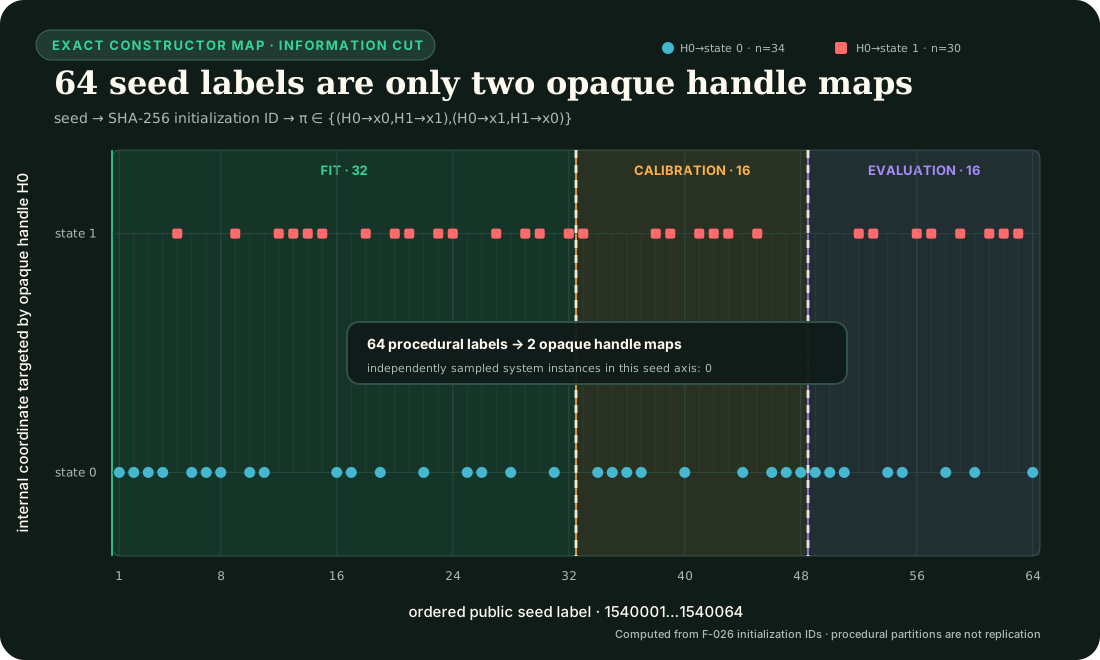
The 64 procedural seed labels map to only two opaque state-handle permutations.

The plotted points are computed from the checked-in initialization-ID and opaque-permutation functions. The colored regions show the access cut; they do not add independent system variation.

The two generic references become mature nulls only after trainable causal state-space and compact recurrent estimators are implemented against the same fixed-parameter packet schema, with no direct plant state, recipe or equation access. Their construction, selection, calibration, failures and fallbacks enter the resource ledger. A later confirmatory comparison needs independently generated held-out system instances and an outer system-family holdout; neither exists in the present five-world bank.

For that later design, the fixed primary endpoint families are mean property log loss in nats and mean dimensionless decision loss. Coverage, selective risk, reliability, compatible-vector coverage and the resource vector are reported alongside them. The earlier Stage-3 wording grouped the two candidate-versus-generic-null contrasts within each endpoint. The later population contract supersedes that weaker boundary and uses the sequentially rejective procedure of Holm (1979), bibliography key holm1979sequential, once across all four fixed endpoint-by-comparator hypotheses at familywise α=0.05\alpha=0.05. Sample size must be powered before private confirmation seeds are created; 16 public evaluation labels are not assumed sufficient.

The closed machine form is rsd-t02-stage3-design.json, validated by rsd-t02-stage3-design.mjs.

Prospective system population and outer-family boundary

The information cut above remains valid, but it is not a population design. The next contract uses the following nesting, from inferentially broad to repeated measurement:

designstructural lineagefamilyindependent instancepacketepisoderealization.\text{design}\supset\text{structural lineage}\supset\text{family} \supset\text{independent instance}\supset\text{packet} \supset\text{episode}\supset\text{realization}.

A procedural seed is only a replay key. A family is one frozen equation template plus a declared parameter distribution. An instance is one accepted parameter vector drawn independently from that family; it is the unit for a fixed-family estimand. Episodes, rows, property coordinates, solver refinements and noise realizations remain nested measurements and never increase the reported independent nn.

This distinction also invalidates a tempting reuse of the current packet. Its nine O0 executions cross τ=0.5,1,2s\tau_*=0.5,1,2\,\mathrm s, while its 26 O1 executions hold τ=1s\tau_*=1\,\mathrm s. One population instance must bind one parameter vector—including one time constant—across every episode. The old mixed-τ\tau packet remains a construction-conformance artifact; a population packet must be regenerated per fixed parameter vector.

The first defensible claim mode is a fixed finite family panel. Visible development families and separately sealed outer-confirmation and outer-transfer families are split by structural lineage, not by recipe label or instance. Related equations, derivations, code siblings and full-panel- equivalent recipes share a leakage group and cannot cross partitions. An outer result therefore generalizes only to the prospectively frozen weighted panel, not to arbitrary future mechanisms. A family-superpopulation claim requires a separate frozen probabilistic family grammar and powers on independently drawn families or lineages.

For coordinate qq, instance ii, family ff and arm aa, first aggregate the coordinate loss inside the instance,

afi=qwqLafiq,dfia,b=afibfi.\ell_{afi}=\sum_q w_q L_{afiq}, \qquad d_{fi}^{a,b}=\ell_{afi}-\ell_{bfi}.

Then form the equal-family weighted contrast

Δ^a,b=fwfdˉfa,b,dˉfa,b=1nfidfia,b,wf=1F.\widehat\Delta^{a,b}=\sum_f w_f\bar d_f^{a,b}, \qquad \bar d_f^{a,b}=\frac{1}{n_f}\sum_i d_{fi}^{a,b}, \qquad w_f=\frac1F.

Resampling occurs over instances within the fixed families; rows are never resampled as independent systems. The prospective power artifact must freeze the smallest effect of interest, alpha, power, family heterogeneity, family and instance counts, abstention coverage, failure disposition and the calculation implementation hash before private responses. The experiment-level success rule applies Holm's procedure across all four fixed endpoint-by-comparator hypotheses at α=0.05\alpha=0.05; controlling two contrasts separately inside each endpoint would not close the cross-endpoint multiplicity boundary.

For equal retained counts in each of FF fixed families, first derive the minimum effective count for one lower-tail contrast:

neff=max{2,fσf2F2(z1α/4+z1βδ)2}.n_{\mathrm{eff}} = \max\left\{ 2, \left\lceil \frac{\sum_f \sigma_f^2}{F^2} \left( \frac{z_{1-\alpha/4}+z_{1-\beta}}{\delta} \right)^2 \right\rceil \right\}.

Here σf2\sigma_f^2 is the development-evaluation variance of the paired system-instance contrast in family ff, δ>0\delta>0 is the minimum relevant improvement magnitude in the endpoint unit, and 1β1-\beta is target power. The α/4\alpha/4 term protects the most conservative first Holm step.

If rr is the prospective probability of pre-response invalid generation and γ\gamma is the registered experiment-level retention assurance, the plotted planned count is instead

nplan=min{mN:Pr ⁣[Binomial(m,1r)<neff]1γF}.n_{\mathrm{plan}} = \min\left\{ m\in\mathbb N: \Pr\!\left[ \operatorname{Binomial}(m,1-r)<n_{\mathrm{eff}} \right] \le \frac{1-\gamma}{F} \right\}.

The Bonferroni allocation on the right guarantees at least γ\gamma retention assurance across the FF family strata without assuming their attrition events are independent. Runtime failures retain their registered in-denominator penalty. The support-coverage floor remains a separate gate and is not silently converted into another sample-size multiplier.
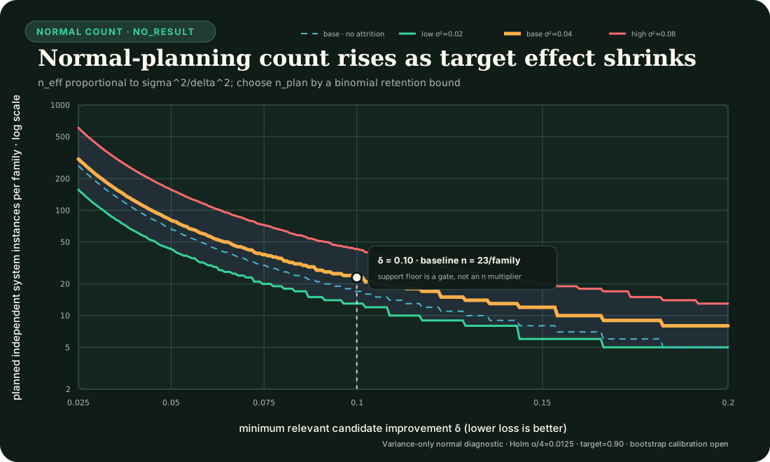
Illustrative prospective independent-system count versus minimum relevant effect under three variance profiles.

The figure is a sensitivity map, not a power result. Its variance profiles are illustrative, so it cannot freeze a sample size. The checked-in calculator requires a development-evaluation variance-artifact hash and exposes every unit, approximation, attrition rule and blocker. A syntactically valid hash does not verify the artifact bytes, role or review, so the calculator always keeps the power-plan release gate open until those bindings are independently validated. The normal calculation also does not establish power for the final bootstrap-tt analyzer: zero-standard-error bootstrap resamples create a data-dependent lower bound

pmin,data=B0+1B+1,p_{\min,\mathrm{data}} = \frac{B_0+1}{B+1},

where BB is the registered resample count and B0B_0 is the number of zero-standard-error resamples conservatively counted as extreme. The analyzer records this bound for every hypothesis and closes its resolution gate only when it can reach the first Holm threshold. A future frozen power artifact must therefore simulate the pilot transcripts through the exact analyzer; variance alone is insufficient.

Synthetic transcript calibration of the exact analyzer

The public diagnostic now performs that simulation step for four declared synthetic scenarios without treating the resulting frequencies as scientific power. For kk events in RR Monte Carlo replicates it reports the smoothed point diagnostic

p~MC=k+1R+1,ΔpMC=1R+1.\widetilde p_{\mathrm{MC}}=\frac{k+1}{R+1}, \qquad \Delta p_{\mathrm{MC}}=\frac{1}{R+1}.

The point smoothing and interval have different jobs. The Wilson score interval is computed for the observed binomial count k/Rk/R; applying Wilson to the artificial pair (k+1,R+1)(k+1,R+1) would give the wrong coverage target and can exclude zero even when a deterministic hostile produces no events.

The generated unit identity uses a DGP-only fingerprint. It binds scenario baselines, attrition, failure probabilities, contrast means and covariances, the simulation key and registered family order. Confidence level, total replicate ceiling, bootstrap count, alpha and endpoint penalties remain in the full configuration/report identity but do not reorder a common generated prefix or change its finite-bootstrap point decision.

The canonical configuration uses R=99R=99 and B=1000B=1000. Its declared synthetic null yields 6 any-rejection events, while the declared minimum-relevant-effect scenario yields 55. The null Wilson Monte Carlo interval, 0.0280.028--0.1260.126, spans the 0.050.05 reference; the alternative interval, 0.4570.457--0.6500.650, is far below the illustrative 0.900.90 target. The two two-instance hostiles each fail the analyzer's bootstrap-resolution gate in all 99 replicates. This rejects plan acceptance; it does not estimate future model power.
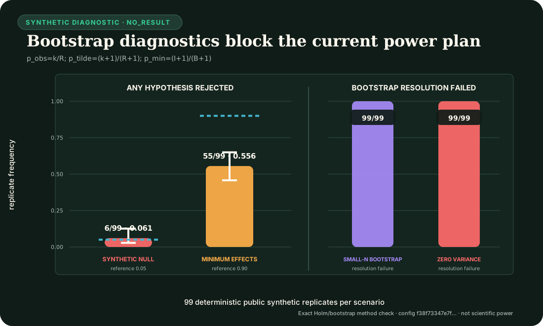
Observed any-rejection frequencies with Wilson Monte Carlo intervals for the declared synthetic null and alternative, beside bootstrap-resolution failure frequencies for two two-instance hostiles.

The executable contract is rsd-t02-pilot-transcript-calibration.json, implemented by rsd-t02-pilot-transcript-calibration.mjs. Closure is narrow: reviewed real pilot bytes and role, an analyzer release hash, jointly frozen effects, target, resampling key and failure penalties, and an accepted planned-count calibration remain open.

The causal-memory coordinate is not primary-scorable in this first population design because the current family bank contains no valid memory-negative lineage. It can become primary only after both values have prospective, lineage-diverse coverage. Outer family templates and truth remain encrypted or evaluator-custodied until the model, calibration, thresholds, analyzer, resource caps and power plan are frozen. A bare public hash is a commitment, not secrecy for a small family search space.

The closed prospective machine form is rsd-t02-population-design.json, validated by rsd-t02-population-contract.mjs.

Exact public fixed-instance construction

The public family registry currently contains the five named equation families only. Four generator-conformance coordinates are crossed with every family, producing 20 metadata artifacts. This count tests deterministic construction; it is not a powered sample size.

For family ff, draw index jj, parameter key kk, and HMAC attempt aa, let

wf,j,k,a=U64BE[HMACKpublic(canon(d,HF,Hf,f,vf,j,k,a))0:8].w_{f,j,k,a} = \operatorname{U64BE} \left[ \operatorname{HMAC}_{K_{\mathrm{public}}} \left( \operatorname{canon}(d,H_{\mathcal F},H_f,f,v_f,j,k,a) \right)_{0:8} \right].

HFH_{\mathcal F} hashes the ordered scientific family definitions only; coverage policy, custody state, packet metadata and generator authority are excluded. HfH_f binds the selected family, including its declared equation- template digest. KpublicK_{\mathrm{public}} is committed replay material rather than a secret. The sole sampled parameter is an integer time constant

τμsDiscreteUniform{500000,,2000000}.\tau_{\mu s}\sim \operatorname{DiscreteUniform}\{500000,\ldots,2000000\}.

With K=1,500,001K=1{,}500{,}001 possible integers and

L=264(264modK),L=2^{64}-(2^{64}\bmod K),

the generator rejects wLw\ge L before applying modulo reduction, then uses

τμs=500000+(wmodK),τs=τμs106 s.\tau_{\mu s}=500000+(w\bmod K), \qquad \tau_s=\frac{\tau_{\mu s}}{10^6}\ \mathrm{s}.

The complete parameter document stores exact numerator, denominator and unit objects. Its digest, the fixed nuisance-interface digest and complete certificate-set digest, including the equation-template digest, enter the canonical system identity. The full registry, population-design bytes and model-source bytes remain separate provenance bindings. The draw index is recorded in the receipt but not in that identity. Every generated packet lists the same parameter digest and τs\tau_s on all 26 unique episodes. A distinct episode-protocol digest binds every schedule, the horizon, integration step, output rate, input bounds, units and interpreter semantics into the packet ID without contaminating the system ID. The generator packet itself contains no trajectories or policy response. A separate fixed-instance conformance runner now materializes its 26 trajectories and causal view. An additive overlay binds a content-addressed 26-projection abstention bundle, executes it in a fresh restricted child, semantically replays the nine responses, and durably resumes an owner-bound fixed-instance ledger. A compact population runner traverses all 20 unique public instances and receipts 520 episodes, 799,240 transcript rows and 180 arm invocations. The integrated execution release composes both layers: one identity-keyed durable instance directory per system and one bounded outer record only after its nine-arm summary is complete and current. Restart tests cover the post-instance/pre-outer crash window and full-panel reopen without duplicating a scientific unit. The outer records contain no endpoints or causal payloads, and the release still does not execute the trained candidate or null policies.

The coverage function counts distinct structural lineages per property value, collapsing the full-panel-equivalent I1-FFL and affine high-pass siblings into one lineage. The frozen minimum is two:
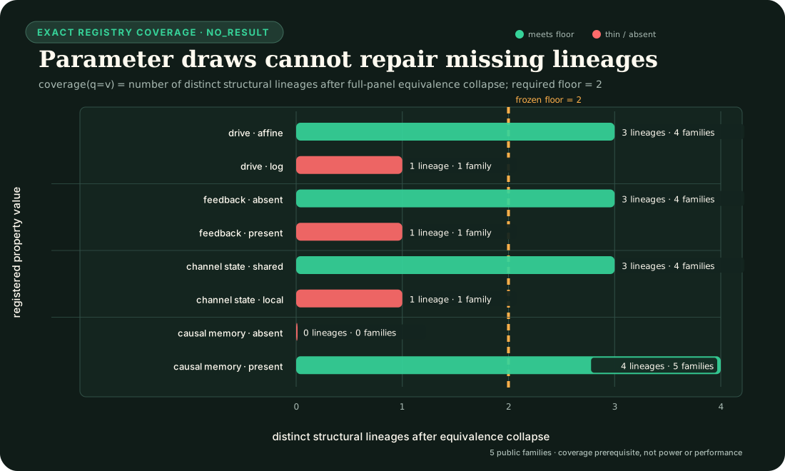
The current public family registry has four property values below the two-lineage floor.

log-fold, feedback-present and channel-local-present each have one lineage; memory-negative has zero. More draws from the current equations cannot close those structural gaps. The closed machine artifacts are the family registry, instance plan, and generator.

Generic-null maturity is a state machine

The executable B-STATE-SPACE and B-RECURRENT policies in the older 35-projection construction bank remain fixed level-one references. Separate deterministic trainable implementations now provide a causal latent state-space prototype and a compact GRU-style prototype. They consume the fixed-instance causal view only through a post-validation adapter and occupy level two; they do not replace the older policy responses. The maturation sequence is:

  1. fixed conformance reference;
  2. trainable public prototype;
  3. fit-frozen development estimator;
  4. calibrated development comparator;
  5. confirmation-frozen mature null; and
  6. confirmation-evaluated run state.

Only level 5 satisfies the population gate. Both current trainable prototypes are at level 2. They emit normalized value posteriors for all three primary coordinates, identifiability probabilities, one coherent joint posterior, support status, a deterministic decide-or-abstain action, reason codes and a typed work ledger, but their probabilities are uncalibrated and their models, resource caps and source/runtime identity are not comparison-frozen. The machine implementations are the prototype module, post-validation adapter, and maturation design.

For instance ii and property qq, a prospective common objective family is

J(θ)=i,qaq[BCE(Iiq,siq)+IiqCE(πiq,piq)]λEilog ⁣(vEiqi(v))+λPLpred(θ)+λRR(θ).J(\theta) = \sum_{i,q}a_q \left[ \operatorname{BCE}(I_{iq},s_{iq}) +I_{iq}\operatorname{CE}(\pi_{iq},p_{iq}) \right] -\lambda_E\sum_i\log\!\left(\sum_{v\in\mathcal E_i}q_i(v)\right) +\lambda_P L_{\mathrm{pred}}(\theta) +\lambda_R R(\theta).

θ\theta is the trainable parameter vector, ii indexes system instances, and qq indexes active property coordinates. Let V\mathcal V be the finite active joint property-vector domain. For each ii, the joint posterior qi:V[0,1]q_i:\mathcal V\to[0,1] is normalized by vVqi(v)=1\sum_{v\in\mathcal V}q_i(v)=1, while the evaluator supplies a nonempty set EiV\varnothing\ne\mathcal E_i\subseteq\mathcal V of compatible vectors. Zero posterior mass on all of Ei\mathcal E_i gives an infinite negative log-mass penalty.

Iiq{0,1}I_{iq}\in\{0,1\} is certified identifiability and siq[0,1]s_{iq}\in[0,1] its predicted probability. If Iiq=1I_{iq}=1, πiq\pi_{iq} is the unique property truth and piqp_{iq} a normalized posterior over the registered values of coordinate qq. If Iiq=0I_{iq}=0, πiq\pi_{iq} is not required and the masked expression is defined as IiqCE(πiq,piq)=0I_{iq}\operatorname{CE}(\pi_{iq},p_{iq})=0. Lpred(θ)L_{\mathrm{pred}}(\theta) and R(θ)R(\theta) are respectively the auxiliary causal-prediction loss and frozen regularizer. They, BCE, CE, and the log-mass term are normalized to dimensionless quantities.

The fit-only training weights satisfy aq0a_q\ge0 and qaq=1\sum_q a_q=1; they are not the common endpoint-aggregation weights wq0w_q\ge0, qwq=1\sum_qw_q=1, which freeze before development evaluation. The coefficients λE>0\lambda_E>0 and λP,λR0\lambda_P,\lambda_R\ge0 are dimensionless and selected inside fit. Predictive horizon, optimizer and stopping rule remain fit-only choices, while the deterministic trial tie-break freezes before any trial outcome exists. Until the causal-memory activation condition passes, Ei\mathcal E_i and qiq_i span the three primary coordinates only; activating the fourth coordinate requires a new contract version, head and calibration.

The exact six-level status, freeze order, common resource requirements and three separate gate scopes are frozen in the null-maturation design. The two trainable-prototype gates and the parameterized isolated durable runner gate are satisfied; seven intrinsic null-maturity gates remain open. Two of ten comparison-release gates—the registry and generator—are also satisfied; the measured-energy meter gate is conditionally applicable only when an energy claim is requested. It is not counted among the 20 mandatory gates for a non-energy comparison. The current non-energy total is therefore five satisfied and 15 open. Affected fitting remains blocked by incomplete lineage coverage, absent sealed outer-family templates, and the absent instance-level fit/calibration/development-evaluation assignment. The exact local runtime closure for the promoted infrastructure gate is recorded in the parameterized runner release.

Calibration and abstention

Probability quality is evaluated with logarithmic loss as a proper scoring rule in the sense reviewed by Gneiting and Raftery (2007), bibliography key gneiting2007scoring. The separate decision loss below encodes this fixture's abstention costs; it is not silently folded into calibration.

For property coordinate qq, let Eq\mathcal E_q be the set of values compatible with the registered observation packet and define

Iq=1[Eq=1].I_q=\mathbb 1[|\mathcal E_q|=1].

When Iq=1I_q=1, let πq\pi_q denote the unique element of Eq\mathcal E_q.

An arm returns a probability P^(Iq=1)\widehat P(I_q=1), a posterior over property values, including posterior mass P^(πq)\widehat P(\pi_q) on that unique compatible value, and either decide or abstain. With probabilities clipped at 101210^{-12}, the calibration loss in nats is

Lcal,q=IqlnP^(Iq=1)(1Iq)ln[1P^(Iq=1)]IqlnP^(πq).L_{\mathrm{cal},q} = -I_q\ln\widehat P(I_q=1) -(1-I_q)\ln[1-\widehat P(I_q=1)] -I_q\ln\widehat P(\pi_q).

When Iq=0I_q=0, the final masked term is defined to be exactly zero; πq\pi_q and P^(πq)\widehat P(\pi_q) are not evaluated.

The decision loss is dimensionless:

Ldec,q={0,Iq=1 and the decision is correct,0.25,Iq=1 and the arm abstains,0,Iq=0 and the arm abstains,1,wrong decision or declaration on a non-singleton set.L_{\mathrm{dec},q} = \begin{cases} 0, & I_q=1\text{ and the decision is correct},\\ 0.25, & I_q=1\text{ and the arm abstains},\\ 0, & I_q=0\text{ and the arm abstains},\\ 1, & \text{wrong decision or declaration on a non-singleton set}. \end{cases}

Coverage, selective risk and reliability remain separate. Sensitivity analyses later vary the identifiable-case abstention cost to 0.10.1 and 0.50.5; they do not replace the primary loss.

The fast boundary layer needs the right norm

The source-qualified stratum uses the nondimensional input-degradation model

τsx˙=uˉx,ϵτsy˙=xuˉy,\tau_s\dot x=\bar u-x, \qquad \epsilon\tau_s\dot y=x-\bar u y,

with τs=1s\tau_s=1\,\mathrm s, uˉ0=1\bar u_0=1, uˉ=2\bar u_*=2, x(0)=uˉ0x(0)=\bar u_0 and y(0)=1y(0)=1. The scaled member uses uˉp=puˉ\bar u_p=p\bar u, xp(0)=puˉ0x_p(0)=p\bar u_0 and yp(0)=1y_p(0)=1.

The primary finite-grid truth is

D,ϵ,p=sup0t8τsyϵ,p(t)yϵ,1(t).D_{\infty,\epsilon,p} = \sup_{0\le t\le8\tau_s} |y_{\epsilon,p}(t)-y_{\epsilon,1}(t)|.

For this registered construction, the associated fast initial-value systems give

Mp=1uˉ0uˉp1pp/(1p)>0,p1,M_p = \left|1-\frac{\bar u_0}{\bar u_*}\right| |p-1|p^{p/(1-p)}>0, \qquad p\ne1,

and a source-shaped finite-ϵ\epsilon bound has the form

D,ϵ,pMpϵN~p.D_{\infty,\epsilon,p} \ge M_p-\epsilon\widetilde N_p.

The protected construction does not infer this asymptotic statement from a finite sweep. It checks the declared generator and bound.

An RMS score measures something else:

D2,ϵ,p=18τs08τsyϵ,p(t)yϵ,1(t)2dt.D_{2,\epsilon,p} = \sqrt{ \frac{1}{8\tau_s} \int_0^{8\tau_s} |y_{\epsilon,p}(t)-y_{\epsilon,1}(t)|^2dt }.

The exact physical-time metric counterexample

eϵ(t)=et/(ϵτs)e_{\epsilon}(t)=e^{-t/(\epsilon\tau_s)}

has

eϵ=1,RMS(eϵ)=ϵτs2T(1e2T/(ϵτs))0.\|e_{\epsilon}\|_{\infty}=1, \qquad \operatorname{RMS}(e_{\epsilon}) = \sqrt{ \frac{\epsilon\tau_s}{2T} \left(1-e^{-2T/(\epsilon\tau_s)}\right) } \longrightarrow0.

A boundary-layer peak remains fixed in the supremum norm while its RMS value falls with epsilon.

The figure is an exact toy norm comparison, not a biological fit or a run of the source-shaped generator.

Fast- and slow-time sampling

The protected grid freezes

ϵ{101,102,103,104,105,106,107},\epsilon\in \{10^{-1},10^{-2},10^{-3},10^{-4},10^{-5},10^{-6},10^{-7}\}, p{0.5,2,4,8,20}.p\in\{0.5,2,4,8,20\}.

The critical initial-layer time is

tϵ,p=ϵτslnp(p1)uˉ.t_{\epsilon,p} = \epsilon\tau_s \frac{\ln p}{(p-1)\bar u_*}.

Every cell samples the union

{ϵτsj128:j=0,,1024}{τsk64:k=0,,512}.\left\{ \epsilon\tau_s\frac{j}{128}:j=0,\ldots,1024 \right\} \cup \left\{ \tau_s\frac{k}{64}:k=0,\ldots,512 \right\}.

The first grid resolves the shrinking boundary layer; the second retains the eight-second slow response. Deduplication leaves at most 1,537 paired rows per cell.

The floor stratum crosses three equation-defined models, seven epsilon values and five scale factors. Besides the singular system above, both controls share

τsx˙=uˉx.\tau_s\dot x=\bar u-x.

The exact-equivariance control reports

y0=uˉx1.y_{0}=\frac{\bar u}{x}-1.

Because the scaled member has uˉp=puˉ\bar u_p=p\bar u and xp=pxx_p=px, its discrepancy is identically zero. The regular-perturbation control reports

yϵ=uˉx1+ϵ(uˉuˉ0).y_{\epsilon} = \frac{\bar u}{x}-1 +\epsilon(\bar u-\bar u_0).

Its scaled-versus-unscaled discrepancy is ϵp1uˉuˉ0\epsilon|p-1||\bar u-\bar u_0| and therefore tends to zero. The three registered models are consequently:

  1. the source-shaped singular construction;
  2. an exact-equivariance zero-floor control; and
  3. a regular-perturbation control whose discrepancy tends to zero.

That is 105 public-development cells and at most 161,385 paired rows. RMS is diagnostic only and cannot establish or refute the supremum floor.

Information firewall

Every actionable arm receives only causal inputs, reported outputs, masks, opaque intervention commands, timestamps and units. Before the arm response is frozen it does not receive:

  1. recipe or equation identity;
  2. semantic state names or the hidden handle permutation;
  3. parameters or evaluator properties;
  4. future samples or future-derived normalization;
  5. the equivalence or separation certificate; or
  6. continuous evaluator truth.

The actionable registry has nine roles:

  1. A-RAW;
  2. B-STATIC-DIV;
  3. B-STREAM;
  4. B-LOG-RATIO;
  5. B-DIFFERENCE;
  6. B-STATE-SPACE;
  7. B-RECURRENT;
  8. C-MECHANISM-BANK; and
  9. C-DUAL.

O-GRAPH is evaluator-only and excluded from parity, tuning, promotion and resource rankings. Public source code does not create confirmation secrecy; a claim-eligible run later needs separately committed sealed seed mapping and custody.

Typed acquisition and computation cost

Do not collapse intervention access and execution into one score. Every arm retains at least:

  1. episodes and sample rows;
  2. serialized observation bytes and input commands;
  3. internal resets, freezes and output clamps;
  4. channel switches and state writes;
  5. scalar operations and transcendental evaluations;
  6. retained-state and parameter bytes;
  7. tuning trials and wall seconds; and
  8. later measured joules, when a calibrated physical protocol exists.

The foundation suggests future caps of one CPU thread, binary64 arithmetic, 16 retained scalars, 512 trainable scalars and 32 tuning trials. They are not active parity claims because actionable algorithms and a complete arm-level parity/resource ledger are absent.

Support and fail-closed cases

Each scientific case retains the six independent support axes already frozen for RSD-T01:

  1. input domain;
  2. transformation family;
  3. instrument range and temporal resolution;
  4. initialization;
  5. causal observation; and
  6. evaluation window.

Valid scientific hostiles include additive offset, near-zero input, clipping, hidden reset, future-aware normalization, channel-state contamination and boundary-layer censoring. Parser, checksum, order or unit failures remain malformed sentinels outside the scientific denominator.

Missing, duplicate, rejected or mixed-initialization transcripts force system abstention and remain visible. A fixed slow-time sampler that misses the protected fast layer is a scientific failure, not a missing-data deletion.

Current authority and kill rules

The machine registry states:

{
  "authority": "contract-foundation-only",
  "partition": "public-development",
  "information_cut_status": "registered-projection-no-secret-custody",
  "comparison_authority": false,
  "result_authority": "NO_RESULT"
}

The registry is the foundation authority, not the execution result. A separate deterministic bounded public-development runtime now consumes the T02-MECH registry to generate all O0/O1 construction episodes, enforce the policy firewall and response commitment, reconstruct evaluator truth, retain typed acquisition/construction/inference ledgers, and validate append-only resume. Its additive Stage 2 commits all nine fixed whole-system policy-conformance responses before evaluator access, with zero inactive placeholders. Every event and analysis remains NO_RESULT; trained or calibrated estimators, mature nulls, comparisons, claim eligibility, O2, T02-FLOOR execution, confirmation, workstation measurement and energy conclusions are absent.

The future T02 comparison is killed if any of the following occurs:

  1. step fit, recipe name or graph access supplies the primary answer;
  2. a declared separating intervention lacks a pairwise certificate;
  3. an arm is rewarded for guessing inside an observational equivalence class;
  4. privileged access is unequal or missing from the cost vector;
  5. RMS or a fixed slow grid substitutes for the registered supremum endpoint;
  6. a finite epsilon sweep is presented as proof of an asymptotic theorem; or
  7. a mechanism-specific bank cannot beat the generic state-space/recurrent null under the same projection and budget.

The current foundation and construction runtime can test equations, exact step matching, operational equivalence, registry closure, schedule semantics, abstention aggregation, replay integrity and temporal-grid coverage. They cannot support architecture superiority, natural-mechanism attribution, workstation readiness or energy efficiency.

Mathematics · 414 words

Horizon-qualified learning outcomes

Scope

This note makes acquisition, retention, transfer, fluency, calibration, motivation, and effort separate outputs. It supports the learning-science audit and the experiment contracts for Candidates 004 and 019. Its evidence boundaries are C-627C-658.

Immediate and retained change

For learner/model ii, skill item jj, and policy mm, let Yijm(t)Y_{ijm}(t) be a score in a declared score unit. Acquisition and retained change are

Aijm=Yijm(tpost)Yijm(tpre),A_{ijm}=Y_{ijm}(t_{\mathrm{post}})-Y_{ijm}(t_{\mathrm{pre}}), Rijm(Δ)=Yijm(tpost+Δ)Yijm(tpre),R_{ijm}(\Delta)= Y_{ijm}(t_{\mathrm{post}}+\Delta)-Y_{ijm}(t_{\mathrm{pre}}),

where retention horizon Δ\Delta is seconds, task events, or another declared clock. A policy can win on AA and lose on R(Δ)R(\Delta).

Transfer is indexed

Let d{0,1,2,3}d\in\{0,1,2,3\} identify preregistered strata: trained form, near variant, changed representation/context, and novel causal composition. Against baseline m0m_0,

Tm(d)=E[Ytransferm,d]E[Ytransferm0,d].T_m(d)= \mathbb E[Y^{\mathrm{transfer}}\mid m,d] -\mathbb E[Y^{\mathrm{transfer}}\mid m_0,d].

Tm(d)T_m(d) uses score units and is reported for every dd. A single mean called “generalization” cannot show which cue, mapping, or composition transferred.

For elapsed time τ\tau seconds, cc correct responses, and nn attempts,

F=cτ[correct tasks s1],e=1cn[1].F=\frac{c}{\tau} \quad[\mathrm{correct\ tasks\ s^{-1}}], \qquad e=1-\frac{c}{n}\quad[1].

Fluency requires the (F,e)(F,e) frontier, not speed alone. Calibration retains item-level confidence before feedback and reports a proper score such as

BS=1Nk=1N(pkyk)2,\operatorname{BS}=\frac{1}{N}\sum_{k=1}^{N}(p_k-y_k)^2,

which is dimensionless for probability pkp_k and binary outcome yky_k.

Skill-local scheduling state

For skill jj, scheduler state is

Lj,t=(a^,r^Δ1:Δq,T^0:3,F^,c^,σ,χ,h,v),\mathcal L_{j,t}= (\hat a,\hat r_{\Delta_1:\Delta_q},\hat T_{0:3}, \hat F,\hat c,\sigma,\chi,h,v),

where a^\hat a is acquisition, r^\hat r retention by target horizon, T^\hat T transfer by stratum, F^\hat F fluency, c^\hat c calibration, σ\sigma support/scaffold state, χ\chi confusability/context, hh intervention history, and vv state/model version. These are estimates with uncertainty, not hidden truth labels.

The next event may retrieve, restudy, vary, compare, explain, fade support, or stop. Difficulty is admissible only when processing succeeds often enough to produce information; failure without interpretable feedback is not useful effort by definition.

Complete cost

Keep raw cost components

cm=(τ,Ne,Nr,Nf,Nh,B,E,HT,HL),\mathbf c_m=(\tau,N_e,N_r,N_f,N_h,B,E,H_T,H_L),

where τ\tau is learner time in seconds; Ne,Nr,Nf,NhN_e,N_r,N_f,N_h are exposure, retrieval, feedback, and hint counts; BB is stored bytes; EE is joules; and HT,HLH_T,H_L are teacher and learner effort in person-seconds. Variable-time mastery, adaptive scheduling, or interactive teaching cannot claim efficiency while receiving uncharged extra attempts or attention.

Falsification boundary

The scheduler loses if tuned spaced repetition, fixed expanding intervals, ordinary knowledge tracing, blocked/random/interleaved schedules, worked examples with fixed fading, hard-example mining, or fixed curriculum match the delayed retention–transfer–cost frontier. A teaching channel loses if a versioned artifact plus tests preserves equal capability across learner/model turnover at lower combined effort.

Mathematics · 1,185 words

Material commitment and realized service

Scope

This note separates information, policy, commitment, physical state, and realized service for resource-bearing AI systems. It instantiates the supply-chain/operations audit and the soil/crop multi-resource audit without treating inventory, routing, buffers, or biological co-limitation as new AI principles. Its evidence boundaries are C-627 and C-659C-678.

Conservation before optimization

For location or module ii over interval tt, physical inventory obeys

Ii,t+1=Ii,t+Reci,t+Ti,tinSi,tTi,toutXi,t,I_{i,t+1}=I_{i,t}+\operatorname{Rec}_{i,t}+T^{\mathrm{in}}_{i,t} -S_{i,t}-T^{\mathrm{out}}_{i,t}-X_{i,t},

where every term is a count, byte quantity, mass, or another single declared unit: on-hand II, receipts Rec\operatorname{Rec}, inbound/outbound transfer TT, issued work SS, and expiry/damage XX. The explicit receipt symbol avoids reusing RR for both receipts and reservations. Forecasts, requests, allocations, and record corrections do not appear as physical flow unless an observed transition links them to it. Filtration, internal recovery, reintroduction, final egress, and storage change likewise remain separate ledger terms (C-1491). A third-body interface inventory also requires generation, transport, transformation, reincorporation, and escape closure before retain/remove optimization (C-1502).

With accepted but unfinished work,

Bi,t+1=[Bi,t+Di,taccSi,t]+,B_{i,t+1}=\left[B_{i,t}+D^{\mathrm{acc}}_{i,t}-S_{i,t}\right]^+,

where backlog BB, accepted demand DaccD^{\mathrm{acc}}, and completion SS use the same work unit. Lost requests require a separate state because they do not remain in BB and may disappear from later demand records.

Resource form and deliverability

For location ii, resource type kk, and interval tt, retain a compartment state

xik,t=(Sbound,Slab,Ssol,Spipe,Qinternal)ik,tT.\mathbf x_{ik,t}= \left( S^{\mathrm{bound}}, S^{\mathrm{lab}}, S^{\mathrm{sol}}, S^{\mathrm{pipe}}, Q^{\mathrm{internal}} \right)^{\mathsf T}_{ik,t}.

SboundS^{\mathrm{bound}} is bound or slow-release stock, SlabS^{\mathrm{lab}} is a labile or exchangeable pool excluding the solution pool, SsolS^{\mathrm{sol}} is material in solution or its transported analogue, SpipeS^{\mathrm{pipe}} is in-transit material inside the declared boundary, and QinternalQ^{\mathrm{internal}} is an already delivered, remobilizable internal pool. The operational compartments are mutually exclusive and use one declared mass, count, or task-native resource unit. Total stock and solution concentration are derived without adding unlike or overlapping states:

Aggregate stock or inflow therefore cannot establish local arrival, uptake, useful consumption, or deficit at the receiver's support (C-1488).

Sik,ttot=1Txik,t,Cik,tsol=Sik,tsolVi,tsol.S^{\mathrm{tot}}_{ik,t}=\mathbf 1^{\mathsf T}\mathbf x_{ik,t}, \qquad C^{\mathrm{sol}}_{ik,t} =\frac{S^{\mathrm{sol}}_{ik,t}}{V^{\mathrm{sol}}_{i,t}}.

VsolV^{\mathrm{sol}} is the declared carrier or solution volume. Reachable stock Sikreachable(t;Φ)S^{\mathrm{reachable}}_{ik}(t;\Phi) and usable stock Uikusable(t;Φ)U^{\mathrm{usable}}_{ik}(t;\Phi) are deadline-qualified functions of this state and the transport/release model, not extra compartments that can be double counted. 1\mathbf 1 is the all-ones vector and T\mathsf T denotes transpose.

The compartment balance is

xik,t+1=Tik,t(θi,t,pHi,t,Θi,t,βi,t)xik,t+aik,teik,tik,t,\mathbf x_{ik,t+1} = \mathbf T_{ik,t}(\theta_{i,t},pH_{i,t},\Theta_{i,t},\beta_{i,t}) \mathbf x_{ik,t} +\mathbf a_{ik,t} -\mathbf e_{ik,t} -\boldsymbol\ell_{ik,t},

where Tik,t\mathbf T_{ik,t} is a dimensionless transition operator for release, sorption/desorption, dissolution, mineralization, and other form changes; θ\theta is volumetric water content, pHpH is the declared logarithmic activity measure, Θ\Theta is temperature on a declared scale, and β\beta is the declared biological or process state. a\mathbf a is externally added material, e\mathbf e is observed service consumption or withdrawal across the boundary, and \boldsymbol\ell is boundary loss. The three vector flow terms are interval-integrated amounts in the same resource unit as x\mathbf x. A resource unit occupies one compartment; transition columns conserve it unless a declared transformation or loss is represented explicitly. Uptake into QinternalQ^{\mathrm{internal}} is an internal transition; it must not also be subtracted as a boundary flow. Internal form changes can conserve an element while changing its deliverability. A lubricant, buffer, cache, or reserve used as an interface mediator remains a typed, regime-qualified resource rather than an automatically beneficial label (C-1499).

Observed uptake over Δt\Delta t is bounded separately from stock:

Uik,tmin ⁣{(Jik,tadv+Jik,tdiff)Δt,Vik,treceiverΔt,Dik,tphysΔt,Sikreachable(t;Φ)},U_{ik,t} \le \min\!\left\{ \left(J^{\mathrm{adv}}_{ik,t}+J^{\mathrm{diff}}_{ik,t}\right)\Delta t, V^{\mathrm{receiver}}_{ik,t}\Delta t, D^{\mathrm{phys}}_{ik,t}\Delta t, S^{\mathrm{reachable}}_{ik}(t;\Phi) \right\},

where UU is observed uptake or receiver acceptance, JadvJ^{\mathrm{adv}} and JdiffJ^{\mathrm{diff}} are non-overlapping advective and diffusive delivery rates, VreceiverV^{\mathrm{receiver}} is receiver uptake or processing capacity, and DphysD^{\mathrm{phys}} is physiological or task demand. Δt\Delta t is the interval duration in seconds. All four right-hand quantities use the same resource amount: the first three are rates in resource units per second integrated over Δt\Delta t, and the fourth is already an amount reachable inside window Φ\Phi. This equation is a service-accounting bound, not a universal soil, crop, or receiver model.

State contract

For service commitment cc, retain

Kc=(Fv,D,A,O,Kres,I,P,C,Q,L,Φ,F,Y,M),\mathcal K_c= (F_v,D,A,O,K^{\mathrm{res}},\mathbf I,P,C,Q,L,\Phi,\mathcal F,Y,M),

where FvF_v is forecast plus vintage, DD observed request, AA admission decision, OO order/release, KresK^{\mathrm{res}} reservation/frozen commitment, I\mathbf I typed on-hand and pipeline inventory by form, age, and condition, PP policy version, CC qualified capacity and common-cause groups, QQ route/queue/qualification state, LL lead-time distribution, Φ\Phi service stage or deadline window, F\mathcal F jointly feasible service set, YY delivered outcome, and MM service-measurement definition. Every field carries event, availability, and decision times when they differ.

The tuple is deliberately not a scalar “available resource.” A valid record does not create physical stock; a route plan does not complete transport; a shipment does not prove correct or timely service. The renal accounting boundary supplies an independent instance of why intermediate throughput is not final service (C-1491).

Jointly executable service

Let service class jj require νjk0\nu_{jk}\ge0 units of resource kk per service unit. At location ii, the currently feasible service set is

Fi(t)={q0:jνjkqjUikusable(t)for every required k,qj=0 outside Φj}.\mathcal F_i(t)= \left\{ \mathbf q\ge0: \sum_j \nu_{jk}q_j \le U^{\mathrm{usable}}_{ik}(t) \quad\text{for every required }k, \quad q_j=0\text{ outside }\Phi_j \right\}.

qjq_j is service units executable within window Φj\Phi_j, and UikusableU^{\mathrm{usable}}_{ik} is the resource amount deliverable within that same window. This bound detects stranded single-resource reservations. It is not a claim that all production functions are fixed-proportion: an experiment must declare partial substitution, internal storage, transformation, and toxicity when they are possible.

For a two-resource factorial experiment, keep the interaction contrast in the same units as the outcome:

Δk=Y11+Y00Y10Y01.\Delta_{k\ell}=Y_{11}+Y_{00}-Y_{10}-Y_{01}.

A positive Δk\Delta_{k\ell} is super-additivity in that experimental context. It does not by itself distinguish simultaneous, independent, or serial co-limitation, nor identify a transport or allocation mechanism.

Service and recovery vectors

Report service as a vector

s=(funit,forder,fOTIF,fbundle,W50,W95,B,Ls,Z,E,Cm,H,Wm),\mathbf s= (f_{\mathrm{unit}},f_{\mathrm{order}},f_{\mathrm{OTIF}}, f_{\mathrm{bundle}},W_{50},W_{95},B,L_s,Z,E,C_m,H,W_m),

where fill/service fractions ff are dimensionless, delays W50,W95W_{50},W_{95} are seconds, fbundlef_{\mathrm{bundle}} is the fraction of commitments whose complete typed resource bundle was executable in its window, backlog BB and lost demand LsL_s use work units, ZZ is stranded reserved resource in a declared resource unit, lifecycle energy EE is joules, monetary cost CmC_m is currency, human work HH is person-seconds, and material waste WmW_m is mass or count. Resource-specific ZZ and WmW_m coordinates remain separate when units differ. Coordinates remain visible even when a declared policy uses weights.

Recovery ends at horizon TRT_R only after backlog, reserve, and next-event service are measured:

R(TR)=(tnominal,tbacklog=0,treserve,ssecond,E,Cm,H,Wm).\mathcal R(T_R)= (t_{\mathrm{nominal}},t_{\mathrm{backlog}=0}, t_{\mathrm{reserve}},\mathbf s_{\mathrm{second}},E,C_m,H,W_m).

Nominal throughput is one timestamp, not the whole recovery state.

For multi-resource systems, the second-event vector also reports residual stock by form, missed service windows, and losses. Late abundance does not retroactively repair a commitment that failed inside its declared window.

Falsification boundary

The held contract loses if typed event sourcing plus inventory reconciliation, queueing/flow models, base-stock or multi-echelon control, stochastic/robust optimization, receding-horizon planning with frozen commitments, and explicit service metrics match its decisions and cost. For soil/crop-derived claims the null stack also includes factorial response surfaces, mechanistic transport-plus-uptake models, balanced-nutrient models, and calibrated crop system simulators. Pooling, supplier count, information sharing, just-in-time operation, co-limitation, structural proliferation, and closed loops receive no default efficiency or resilience credit.

Mathematics · 1,052 words

Measurement contracts, uncertainty, and invalidation

Scope

This note defines the minimum mathematics needed to turn an indication into a decision-bearing result. It connects the metrology audit, Candidate 014, and the energy model. It does not replace a domain-specific measurement procedure.

Result record

For one measured quantity, retain

M=(Y,y^,uc,U,k,Q,P,C,E,S,D,V,t0,t1),\mathcal M=(Y,\hat y,u_c,U,k,\mathcal Q,\mathcal P,\mathcal C, \mathcal E,\mathcal S,\mathcal D,\mathcal V,t_0,t_1),

where:

SymbolMeaningUnit or declaration
YYmeasurand: quantity intended to be measuredphysical unit or named reference scale
y^\hat yvalue estimate attributed to YYsame unit as YY
ucu_ccombined standard uncertaintysame unit as YY
UUexpanded uncertaintysame unit as YY
kkcoverage factor such that U=kucU=ku_cdimensionless
Q\mathcal Qobject, population, component, state, location, and conditionstyped metadata
P\mathcal Pmeasurement procedure and modelversioned identifier
C\mathcal Ccalibration chain, references, corrections, and validity scopedependency record
E\mathcal Eenvironment and influence quantitiesvalues with units
S\mathcal Ssampling, selection, missingness, and association contractprobability/model record
D\mathcal Ddecision rule, tolerance, guard band, and risk allocationversioned rule
V\mathcal Vdata, software, instrument, certificate, and transformation provenancedependency graph
t0,t1t_0,t_1start and end of the supported intervalseconds on a named time basis

The tuple is incomplete when a field that can alter the downstream decision is missing. A confidence score alone cannot represent these distinct dependencies (C-519C-524).

Measurement model and dimensional validity

Let

Y=f(X1,,Xn),Y=f(X_1,\ldots,X_n),

where input quantity XiX_i has unit [Xi][X_i] and YY has unit [Y][Y]. Every additive term produced by ff must have unit [Y][Y]. Software, coefficients, numerical precision, and preprocessing that implement ff are part of P\mathcal P. A coefficient of friction is therefore not portable without its interface pair, load/motion state, environment, procedure, support, and history (C-1497).

For estimates xix_i, first-order covariance propagation gives

uc2(y^)=i=1nj=1ncicju(xi,xj),ci=fXix1,,xn.u_c^2(\hat y)= \sum_{i=1}^{n}\sum_{j=1}^{n} c_i c_j u(x_i,x_j), \qquad c_i=\left.\frac{\partial f}{\partial X_i}\right|_{x_1,\ldots,x_n}.

cic_i has unit [Y]/[Xi][Y]/[X_i] and covariance u(xi,xj)u(x_i,x_j) has unit [Xi][Xj][X_i][X_j], so every summand has unit [Y]2[Y]^2. Removing off-diagonal terms asserts independence; it is not a harmless simplification when calibration, clock, environment, preprocessing, prior, or training data are shared (C-525, C-533). For nonlinear or discontinuous models, propagate sampled input distributions and report empirical interval coverage.

Error, correction, and coverage

Given reference value yrefy_{\mathrm{ref}},

e=y^yref,c=e^,y^corr=y^+c.e=\hat y-y_{\mathrm{ref}}, \qquad c=-\hat e, \qquad \hat y_{\mathrm{corr}}=\hat y+c.

Error ee, correction cc, and corrected estimate y^corr\hat y_{\mathrm{corr}} have unit [Y][Y]. The estimated correction remains uncertain. Expanded uncertainty is

U=kuc,U=k u_c,

where kk is dimensionless. A stated kk does not by itself establish a coverage probability; the distributional method and achieved coverage must be reported (C-524, C-526).

Repeatability and reproducibility

For replicate result ylorsy_{lors} from location ll, operator oo, run rr, and system ss, a variance-component null is

ylors=μ+Ll+Oo+Rr(lo)+Ss+ϵlors.y_{lors}=\mu+L_l+O_o+R_{r(lo)}+S_s+\epsilon_{lors}.

μ\mu and every random effect have unit [Y][Y]; their variances have unit [Y]2[Y]^2. The design declares which factors are fixed or random and which are confounded. A short run with one system estimates repeatability, not broad reproducibility (C-527, C-528).

Decision rules and guard bands

Let specification require YTY\le T, where TT has unit [Y][Y]. A simple guarded acceptance rule is

accept if y^+gUT,\text{accept if }\hat y+gU\le T,

where guard multiplier g0g\ge0 is dimensionless. Increasing gg generally reduces false acceptance while increasing false rejection. Choose gg from a declared loss or risk allocation; do not hide that choice inside “confidence.” The rule version, tolerance version, uncertainty method, and cost owner are dependencies of the decision (C-531).

Drift and recalibration

Represent indication drift relative to the last accepted calibration as

d(t)=ycheck(t)yref(t),d(t)=y_{\mathrm{check}}(t)-y_{\mathrm{ref}}(t),

where dd, check-standard result ychecky_{\mathrm{check}}, and reference value yrefy_{\mathrm{ref}} share unit [Y][Y]. The review policy is a function

πcal=π(ht,rt,ut,ct,et),\pi_{\mathrm{cal}}= \pi(h_t,r_t,u_t,c_t,e_t),

where hth_t is calibration/check history, rtr_t is decision risk, utu_t is current uncertainty, ctc_t is calibration cost, and ete_t is equipment and environment state. Inputs keep their native units; π\pi returns a categorical action such as continue, check, restrict, recalibrate, or quarantine. A calendar interval alone is not evidence of stability (C-532).

Dependency invalidation

Let a directed acyclic graph G=(V,E)G=(V,E) contain calibration, raw-data, software, model, transformation, result, and decision versions. Edge (a,b)E(a,b)\in E means that node bb depends on node aa. If dependency aa changes or fails review, its invalidation cone is

I(a)={vV:av},\mathcal I(a)=\{v\in V: a\leadsto v\},

where ava\leadsto v denotes a directed path and I(a)\mathcal I(a) is a set of version identifiers. Each affected node is re-evaluated, superseded, restricted, or withdrawn; provenance alone does not decide which action is correct (C-534, C-535).

Energy-measurement instantiation

For sampled power PmP_m at time tmt_m with interval Δtm\Delta t_m,

E^=m=1MPmΔtm,\hat E=\sum_{m=1}^{M}P_m\Delta t_m,

where PmP_m is W, Δtm\Delta t_m is s, and E^\hat E is J. The model must name the electrical boundary, voltage/current/phase calibration, bandwidth, anti-aliasing, clock alignment, integration rule, missing-sample policy, warm-up, idle allocation, retries, useful outputs, and facility attribution. Uncertainty propagates through the integration model with shared meter, coefficient, and clock covariance retained.

Compare candidate CC and baseline BB only after both satisfy the same quality, risk, latency, and workload envelope. For paired run rr,

Δer=EC,rNq,C,rEB,rNq,B,r,\Delta e_r= \frac{E_{C,r}}{N_{q,C,r}}- \frac{E_{B,r}}{N_{q,B,r}},

where energies are J, NqN_q is a qualified-event count, and Δer\Delta e_r is J/qualified event. Report absolute values, paired effect, coverage, and all failed or rejected runs. A software counter or narrow device boundary may rank systems differently from calibrated end-to-end measurement; the direction is an empirical question (C-536).

Falsification conditions

Reject the cross-layer composition as a distinct systems contribution if:

  1. a complete conventional metrology, statistics, and content-addressed provenance stack matches its coverage and stale-decision frontier;
  2. it improves results only by receiving extra sensors, calibration runs, compute, storage, or analyst time;
  3. dependencies are recorded but do not trigger correct downstream action;
  4. uncertainty intervals become narrower while empirical coverage worsens;
  5. shared dependencies are counted as independent evidence; or
  6. the metadata and review burden costs more than the errors or work it avoids.

Mathematics · 763 words

Budgeted memory lifecycle

Purpose

Turn selective replay, consolidation, and forgetting into a costed decision problem. This note specifies a testable controller; it does not claim that its score is biologically implemented or optimal.

Memory items and actions

At maintenance cycle tt, the candidate memory set is Mt\mathcal{M}_t. Each item iMti \in \mathcal{M}_t may receive one action

ai,tA={defer,replay,merge,externalize,weaken,delete}.a_{i,t} \in \mathcal{A} = \{\text{defer},\text{replay},\text{merge},\text{externalize}, \text{weaken},\text{delete}\}.

The action is versioned. weaken and delete are invalid unless an external provenance record or explicit retention-policy exception exists.

Expected utility

For item ii and action aa, estimate

Gi,a,t=ΔL^i,a,t+λRΔR^i,a,t+λSΔS^i,a,tλDD^i,a,t,G_{i,a,t} = \widehat{\Delta L}_{i,a,t} + \lambda_R \widehat{\Delta R}_{i,a,t} + \lambda_S \widehat{\Delta S}_{i,a,t} - \lambda_D \widehat{D}_{i,a,t},

where:

  • ΔL^i,a,t\widehat{\Delta L}_{i,a,t} is the predicted reduction in future task loss relative to defer (dimensionless loss units);
  • ΔR^i,a,t\widehat{\Delta R}_{i,a,t} is the predicted reduction in a declared risk metric (risk units);
  • ΔS^i,a,t\widehat{\Delta S}_{i,a,t} is the predicted improvement in schema-consistent transfer (dimensionless score units);
  • D^i,a,t\widehat{D}_{i,a,t} is predicted destructive-action harm, including rare memory loss and provenance failure (harm units);
  • λR\lambda_R has units loss/risk;
  • λS\lambda_S has units loss/score; and
  • λD\lambda_D has units loss/harm.

The terms cannot be added before the conversion coefficients and evaluation sets are declared. Novelty, uncertainty, reward surprise, familiarity, and interference are features used to estimate these outcomes, not interchangeable units of utility.

Resource model

For each candidate action, predict:

  • Ei,a,tE_{i,a,t} — energy in joules;
  • Bi,a,tB_{i,a,t} — data moved in bytes;
  • Ti,a,tT_{i,a,t} — wall time in seconds; and
  • Wi,a,tW_{i,a,t} — slow-model optimizer updates (count).

The scheduler selects binary variables xi,a,t{0,1}x_{i,a,t} \in \{0,1\}:

maxxiMtaAxi,a,t(Gi,a,tλEEi,a,t)\max_x \sum_{i \in \mathcal{M}_t} \sum_{a \in \mathcal{A}} x_{i,a,t} \left(G_{i,a,t} - \lambda_E E_{i,a,t}\right)

subject to

axi,a,t=1i,\sum_a x_{i,a,t} = 1 \quad \forall i, i,axi,a,tEi,a,tEtmax,i,axi,a,tBi,a,tBtmax,\sum_{i,a} x_{i,a,t}E_{i,a,t} \le E_t^{\max}, \qquad \sum_{i,a} x_{i,a,t}B_{i,a,t} \le B_t^{\max}, i,axi,a,tTi,a,tTtmax,i,axi,a,tWi,a,tWtmax.\sum_{i,a} x_{i,a,t}T_{i,a,t} \le T_t^{\max}, \qquad \sum_{i,a} x_{i,a,t}W_{i,a,t} \le W_t^{\max}.

λE\lambda_E has units loss/joule. The four budgets prevent a scheduler from appearing efficient by hiding memory traffic, time, or optimizer work behind a single energy proxy.

This is a multiple-choice multidimensional knapsack problem when predictions are fixed. The first experiment need not solve it exactly; greedy, learned, and standard replay priorities are compared under the same budgets.

The illustrative single-item price envelope shows how the upper admissible action can change with λE\lambda_E. Its gains, costs, and selected actions are hypothetical and are not a fitted policy.

Reconsolidation gate

Retrieval produces a candidate branch rather than mutating the stored item in place. Let mi,tm_{i,t} be a calibrated mismatch statistic and θt\theta_t a gate:

zi,t=1[mi,t>θt].z_{i,t} = \mathbb{1}[m_{i,t} > \theta_t].

If zi,t=0z_{i,t}=0, the item remains read-only. If zi,t=1z_{i,t}=1, an update branch is allowed but promotion still requires regression and provenance tests. Because the exact biological prediction-error boundary is disputed under C-040, θt\theta_t is an experimental variable, not a biological constant.

Required ablations are:

  1. always read-only;
  2. always writable on retrieval;
  3. fixed mismatch threshold;
  4. calibrated risk-dependent threshold; and
  5. explicit source-version change rather than inferred mismatch.

Schema-fit gate

Let si,ts_{i,t} be schema-fit estimated on a held-out structural probe and qi,tq_{i,t} be shortcut risk. A candidate may receive a cheaper merge path only when

si,tτsandqi,tτq.s_{i,t} \ge \tau_s \quad \text{and} \quad q_{i,t} \le \tau_q.

The thresholds τs\tau_s and τq\tau_q are calibrated on validation streams with both compatible items and deceptive near-matches. Training loss alone is not a schema-fit measure.

Measurement protocol

Report both realized and predicted quantities:

QuantityUnitBoundary
replay compute energyJaccelerator or node, declared per run
memory trafficbytehost–device and device memory reported separately
maintenance timeswall clock, including scheduler
optimizer workupdate countslow-model updates only
retentiontask metric by item agefixed evaluation stream
adaptationevents or seconds to thresholdafter declared change point
obsolete intrusionerror count/rateoutdated association probes
destructive erroritem count/ratedeleted state later shown necessary
provenance recoveryfractiondeleted items reconstructable from source

Calibration error between predicted GG and realized outcome is itself a core result. A scheduler that makes good-looking choices only after seeing future tests is invalid.

Falsification

The memory-lifecycle controller fails its first test if a conventional single-priority or reservoir baseline matches its quality–risk–energy frontier, if scheduling overhead consumes the saved replay budget, or if destructive errors exceed the declared safety bound.

Mathematics · 3,073 words

Mission-profile-qualified device reliability contract

This note defines the quantitative boundary for Fixture F-008. It operationalizes the durable result of the semiconductor device and circuit reliability audit: accepted service must be evaluated against the actual mission profile of a variable and aging physical population, with mechanism-qualified extrapolation, explicit correction and retirement, and complete lifecycle ledgers.

  • Status: fixture mathematics; no new principle or candidate
  • Comparison unit: one preregistered service interval and its physical cohort
  • Primary rule: never infer recovery, reliability, or efficiency from task score, monitor output, accelerated stress, or component energy alone

Physical identity and time base

For service episode ee at sample time tt, seal the identity envelope

Ie,t=(l,w,d,b,p,h,s,e,t),I_{e,t}=(l,w,d,b,p,h,s,e,t),

where ll identifies a fabrication lot, ww a wafer, dd a die, bb a physical block or array, pp a package and board path, hh a hardware and firmware version, ss a site or facility, ee an episode, and tt elapsed time [s] from a declared clock origin. All identifiers are immutable byte strings. Replacement, repair, reprogramming, remapping, firmware change, or calibration creates a new versioned identity link; it does not overwrite history.

Let Δtn=tn+1tn\Delta t_n=t_{n+1}-t_n [s] be sample interval nn. The actual mission profile over interval [0,Te][0,T_e] is

Me={un,Vn,fn,Tn,Jn,an,ϕn,D˙nion,cn,rn,Δtn}n=0Ne1,M_e=\left\{ u_n,V_n,f_n,T_n,J_n,a_n,\phi_n,\dot D^{\mathrm{ion}}_n,c_n,r_n,\Delta t_n \right\}_{n=0}^{N_e-1},

where unu_n is workload class [class], VnV_n supply or terminal voltage [V], fnf_n clock or operation rate [Hz], TnT_n measured absolute temperature [K], JnJ_n current density [A m2^{-2}], ana_n switching or access activity [dimensionless], ϕn\phi_n particle flux [particle m2^{-2} s1^{-1}], D˙nion\dot D^{\mathrm{ion}}_n ionizing dose rate [Gy s1^{-1}], cnc_n cooling state [state], rnr_n route and protection state [state], and NeN_e is the number of intervals [interval]. Te=nΔtnT_e=\sum_n\Delta t_n is episode duration [s]. Commanded voltage, nominal temperature, or benchmark label cannot substitute for the measured histories.

The workload record is further resolved as

un=(qn,Nnop,Bnmove,Nnwrite,yn),u_n=(q_n,N_n^{\mathrm{op}},B_n^{\mathrm{move}},N_n^{\mathrm{write}},y_n),

where qnq_n is requested service type [type], NnopN_n^{\mathrm{op}} is operation count [operation], BnmoveB_n^{\mathrm{move}} is bytes moved [byte], NnwriteN_n^{\mathrm{write}} is write or program count [write], and yny_n is the required quality and safety envelope [contract].

Latent physical state and observable evidence

Let the latent device state be

zn=(θ,Dnperm,Rnrev,Wn,Fn,Qnres),z_n=(\theta,D_n^{\mathrm{perm}},R_n^{\mathrm{rev}},W_n, \mathcal F_n,Q_n^{\mathrm{res}}),

where θ\theta is the time-zero physical parameter vector in declared native units, DnpermD_n^{\mathrm{perm}} is cumulative irreversible damage [damage unit], RnrevR_n^{\mathrm{rev}} is reversible degradation [damage unit], WnW_n is consumed write, cycle, or stress endurance [cycle or declared wear unit], Fn\mathcal F_n is latent fault state [state], and QnresQ_n^{\mathrm{res}} is remaining repair, spare, timing, thermal, and correction reserve [declared reserve unit]. A dimensionless normalized representation is allowed only after every component scale is fixed.

The physical transition law is

zn+1=gk(zn,Me,n,αk,Γk,ξn),z_{n+1}=g_k(z_n,M_{e,n},\alpha_k,\Gamma_k,\xi_n),

where gkg_k is a mechanism-qualified transition model, kk indexes a physical mechanism, Me,nM_{e,n} is the mission-profile slice, αk\alpha_k is a vector of mechanism parameters in declared native units, Γk\Gamma_k contains interaction coefficients, and ξn\xi_n is process noise in the units of zz. A model that mixes mechanisms must identify kk or explicitly carry a mixture state.

Observed telemetry is

on=h(zn,Me,n,βvn)+ϵn,ϵnpϵ,vn,o_n=h(z_n,M_{e,n},\beta_{v_n})+\epsilon_n, \qquad \epsilon_n\sim p_{\epsilon,v_n},

where ono_n is the observation vector in sensor-native units, hh is the measurement function, βvn\beta_{v_n} is calibration state under calibration version vnv_n, and pϵ,vnp_{\epsilon,v_n} is the version-qualified noise law. Calibration state has covariance Σnβ\Sigma^{\beta}_n in squared native units.

Define observation availability mn,j{0,1}m_{n,j}\in\{0,1\} for channel jj and censoring bounds Ln,jL_{n,j} and Un,jU_{n,j} in the channel's native unit. The observation record is

On=(on,mn,Ln,Un,vn,Σnβ,anev),O_n=(o_n,m_n,L_n,U_n,v_n,\Sigma^{\beta}_n,a^{\mathrm{ev}}_n),

where anev=tntnlastqualifieda^{\mathrm{ev}}_n=t_n-t_n^{\mathrm{last\,qualified}} is evidence age [s]. Adaptive physical interfaces require the same explicit latent inventory, mode, hysteresis, depletion, health, evidence-age, and fallback state; an “adaptive” label is not an observation (C-1504). For a right-censored lifetime tif>Cit_i^{\mathrm f}>C_i, unit ii contributes

Li=S(CiMi),\mathcal L_i=S(C_i\mid M_i),

where CiC_i is censor time [s], SS is survival probability [dimensionless], and MiM_i is the unit's observed mission profile. A failed unit with failure time tift_i^{\mathrm f} [s] and classified mechanism kik_i contributes

Li=λki(tifMi)S(tifMi),\mathcal L_i=\lambda_{k_i}(t_i^{\mathrm f}\mid M_i) S(t_i^{\mathrm f}\mid M_i),

where λki\lambda_{k_i} is mechanism-specific hazard [s1^{-1}]. Missing and censored records are represented in the likelihood; they are not imputed as healthy observations.

Hierarchical variation, yield, and leakage control

For parameter qq measured at lot ll, wafer ww, die dd, and block bb, use the hierarchical decomposition

θl,w,d,b,q=μq+Ll,q+Wl,w,q+Dl,w,d,q+Bl,w,d,b,q+ηl,w,d,b,q,\theta_{l,w,d,b,q}=\mu_q+L_{l,q}+W_{l,w,q}+D_{l,w,d,q} +B_{l,w,d,b,q}+\eta_{l,w,d,b,q},

where μq\mu_q is the population mean, Ll,qL_{l,q} the lot effect, Wl,w,qW_{l,w,q} the wafer effect, Dl,w,d,qD_{l,w,d,q} the die effect, Bl,w,d,b,qB_{l,w,d,b,q} the local block effect, and ηl,w,d,b,q\eta_{l,w,d,b,q} measurement residual, all in the native unit of qq. Spatial covariance and gradients are modeled explicitly when present.

Let Ai,q=1A_{i,q}=1 when physical unit ii satisfies acceptance criterion qq and Ai,q=0A_{i,q}=0 otherwise. Joint accepted yield is

Y^joint=1Nfabi=1Nfabq=1QAi,q,\widehat Y_{\mathrm{joint}}= \frac{1}{N_{\mathrm{fab}}} \sum_{i=1}^{N_{\mathrm{fab}}} \prod_{q=1}^{Q} A_{i,q},

where NfabN_{\mathrm{fab}} is the number of fabricated units [unit], QQ is the number of jointly required criteria [criterion], and Y^joint\widehat Y_{\mathrm{joint}} is dimensionless. Failed, untestable, unpackageable, and discarded dies remain in NfabN_{\mathrm{fab}}.

For a die area AdieA_{\mathrm{die}} [m2^2] and random killer-defect density D0D_0 [defect m2^{-2}], the Poisson yield null is

YP=exp(AdieD0),Y_{\mathrm P}=\exp(-A_{\mathrm{die}}D_0),

where YPY_{\mathrm P} is dimensionless. More flexible clustering models may replace this null only with held-out wafer and lot evidence.

Competing mechanisms and mission-profile damage

For KK competing mechanisms, total hazard is

λ(tM)=k=1Kλk(tM),\lambda(t\mid M)=\sum_{k=1}^{K}\lambda_k(t\mid M),

and survival through time tt is

S(tM)=exp ⁣[0tλ(τM)dτ],S(t\mid M)= \exp\!\left[-\int_0^t\lambda(\tau\mid M)\,\mathrm d\tau\right],

where λ\lambda and every λk\lambda_k have unit s1^{-1}, tt and τ\tau have unit s, and SS is dimensionless. Cause-specific cumulative incidence is

Fk(tM)=0tS(τM)λk(τM)dτ,F_k(t\mid M)= \int_0^t S(\tau^-\mid M)\lambda_k(\tau\mid M)\,\mathrm d\tau,

where FkF_k is dimensionless and τ\tau^- denotes the instant before τ\tau.

For a monotone damage proxy, define

Dk(t)=0trk ⁣(V(τ),T(τ),J(τ),a(τ),ϕ(τ),u(τ))dτ,D_k(t)=\int_0^t r_k\!\left(V(\tau),T(\tau),J(\tau),a(\tau),\phi(\tau),u(\tau)\right) \,\mathrm d\tau,

where rkr_k is mechanism-kk damage rate [damage unit s1^{-1}] and DkD_k is accumulated damage [damage unit]. This integral is evaluated on actual telemetry, not on mean voltage or mean temperature. Endpoint-matched wear histories can therefore carry different mechanism, transition, repair, and remaining-service state (C-1500).

The equal-mean mission-history illustration uses hypothetical Arrhenius parameters to visualize this nonlinearity; it is not calibrated device damage.

An Arrhenius acceleration factor between use temperature TuT_u [K] and stress temperature TsT_s [K] is

AFT=exp ⁣[EakB(1Tu1Ts)],AF_T=\exp\!\left[ \frac{E_a}{k_{\mathrm B}} \left(\frac{1}{T_u}-\frac{1}{T_s}\right) \right],

where EaE_a is activation energy [eV], kBk_{\mathrm B} is Boltzmann's constant [eV K1^{-1}], and AFTAF_T is dimensionless. The electromigration lifetime null is

t50=AEMJnEMexp ⁣(Ea,EMkBT),t_{50}=A_{\mathrm{EM}}J^{-n_{\mathrm{EM}}} \exp\!\left(\frac{E_{a,\mathrm{EM}}}{k_{\mathrm B}T}\right),

where t50t_{50} is median failure time [s], AEMA_{\mathrm{EM}} has the compound unit required to yield seconds, JJ is current density [A m2^{-2}], nEMn_{\mathrm{EM}} is dimensionless, and Ea,EME_{a,\mathrm{EM}} is activation energy [eV]. The fitted range, waveform, geometry, and failure criterion travel with every estimate.

Radiation-induced upset rate for sensitive regions jj is

RSEU=j0ϕj(E)σj(E)dE,R_{\mathrm{SEU}}= \sum_j\int_0^\infty \phi_j(E)\sigma_j(E)\,\mathrm dE,

where EE is particle energy [J or eV, declared consistently], ϕj(E)\phi_j(E) is differential flux [particle m2^{-2} s1^{-1} energy1^{-1}], σj(E)\sigma_j(E) is upset cross-section [m2^2/bit or m2^2/device], and RSEUR_{\mathrm{SEU}} is upset rate [bit1^{-1} s1^{-1} or device1^{-1} s1^{-1}].

For mechanisms kk and rr, interaction departure is

Δk,r(M)=Lk+r(M)Lk(M)Lr(M)+L0(M),\Delta_{k,r}(M)= L_{k+r}(M)-L_k(M)-L_r(M)+L_0(M),

where Lk+rL_{k+r} is loss under combined stress, LkL_k and LrL_r are losses under each stress alone, and L0L_0 is unstressed loss, all in the same task or physical unit. Δk,r=0\Delta_{k,r}=0 is the additive null; the sign and uncertainty of Δk,r\Delta_{k,r} must be reported rather than absorbed into an unspecified "aging" variable.

Accelerated-test support and extrapolation

Let xstressx^{\mathrm{stress}} be the vector of stress covariates in their normalized, preregistered coordinates and let Strain\mathcal S_{\mathrm{train}} be the support of the accelerated-test design. Define support distance

dsup(x)=infxStrainxxΣ1,d_{\mathrm{sup}}(x)= \inf_{x'\in\mathcal S_{\mathrm{train}}} \left\|x-x'\right\|_{\Sigma^{-1}},

where Σ\Sigma is a fixed covariance or scale matrix, vΣ1=vΣ1v\|v\|_{\Sigma^{-1}}=\sqrt{v^{\top}\Sigma^{-1}v} is dimensionless Mahalanobis distance, and dsupd_{\mathrm{sup}} is dimensionless. A prediction is out of support when dsup(x)>dmaxd_{\mathrm{sup}}(x)>d_{\max} for preregistered dimensionless threshold dmaxd_{\max}.

For a nominal (1α)(1-\alpha) survival interval [S^iL(t),S^iU(t)][\widehat S_i^L(t),\widehat S_i^U(t)], empirical interval coverage is

C^S(t)=1Nholdi=1Nhold1 ⁣[Si(t)[S^iL(t),S^iU(t)]],\widehat C_S(t)= \frac{1}{N_{\mathrm{hold}}} \sum_{i=1}^{N_{\mathrm{hold}}} \mathbb 1\!\left[ S_i(t)\in[\widehat S_i^L(t),\widehat S_i^U(t)] \right],

where α\alpha, SiS_i, and C^S\widehat C_S are dimensionless, NholdN_{\mathrm{hold}} is held-out unit count [unit], and 1\mathbb 1 is the indicator function. Mechanism transitions, failure-analysis disagreement, or false-safe predictions invalidate extrapolation even when aggregate error is small.

Thermal, electrical, and wear coupling

For thermal node vector T(t)T(t) [K], the lumped electrothermal null is

CthdTdt+Gth(TTamb)=P(t),C_{\mathrm{th}}\frac{\mathrm dT}{\mathrm dt} +G_{\mathrm{th}}(T-T_{\mathrm{amb}})=P(t),

where CthC_{\mathrm{th}} is thermal-capacitance matrix [J K1^{-1}], GthG_{\mathrm{th}} is thermal-conductance matrix [W K1^{-1}], TambT_{\mathrm{amb}} is ambient-temperature vector [K], and P(t)P(t) is dissipated power vector [W]. Routing comparisons use measured spatial T(t)T(t) and P(t)P(t).

Dynamic switching energy for operation class qq is

Edyn,q=NqαqCqVq2,E_{\mathrm{dyn},q}=N_q\alpha_q C_q V_q^2,

where NqN_q is operation count [operation], αq\alpha_q is activity factor [dimensionless], CqC_q is effective switched capacitance [F/operation], VqV_q is voltage [V], and Edyn,qE_{\mathrm{dyn},q} is energy [J]. Leakage, regulation, clocking, memory, transfer, monitoring, correction, thermal control, and idle energy are separate terms.

For physical element jj, normalized wear evolves as

wj(t+Δt)=wj(t)+Δxj(t)Xjend,w_j(t+\Delta t)=w_j(t)+ \frac{\Delta x_j(t)}{X^{\mathrm{end}}_j},

where wjw_j is dimensionless consumed endurance, Δxj\Delta x_j is stress, write, or cycle increment [wear unit], and XjendX^{\mathrm{end}}_j is measured endurance capacity [same wear unit]. Element jj is exhausted when wj1w_j\ge 1, unless a stricter registered threshold applies.

Separate native margin, reversible recovery, and compensation as

mjobs(t)=mj0djperm(t)djrev(t)+cjcomp(t),m^{\mathrm{obs}}_j(t)=m^{0}_j -d^{\mathrm{perm}}_j(t)-d^{\mathrm{rev}}_j(t) +c^{\mathrm{comp}}_j(t),

where mjobsm^{\mathrm{obs}}_j, mj0m^0_j, permanent loss djpermd^{\mathrm{perm}}_j, reversible loss djrevd^{\mathrm{rev}}_j, and compensation cjcompc^{\mathrm{comp}}_j share the same physical margin unit, such as volts or seconds. A reduction in djrevd^{\mathrm{rev}}_j is recovery; an increase in cjcompc^{\mathrm{comp}}_j is adaptation. They are never scored as the same event.

Fault geometry and the soft/hard firewall

Let every fault event carry type

fi=(gi,i,τi,pi,ci,xi),f_i=(g_i,\ell_i,\tau_i,p_i,c_i,x_i),

where gig_i is spatial geometry [bit, word, bank, chip, route, or domain], i\ell_i is persistence [s], τi\tau_i is occurrence time [s], pip_i is physical or injected provenance [class], cic_i is common-cause identifier [class], and xix_i is external-side-effect state [state].

The firewall outcome is one of

Yifw{CE,DUE,SDC,MC,ESC},Y_i^{\mathrm{fw}}\in \{\mathrm{CE},\mathrm{DUE},\mathrm{SDC},\mathrm{MC},\mathrm{ESC}\},

where CE is corrected error, DUE is detected uncorrectable error, SDC is silent data corruption, MC is miscorrection, and ESC is escaped unsafe side effect. Each is counted in events [event]. For NtxN_{\mathrm{tx}} protected transactions,

Ry=NyNtx,R_y=\frac{N_y}{N_{\mathrm{tx}}},

where NyN_y is count [event] of firewall outcome yy, and RyR_y is rate [event/transaction]. SDC and ESC are never merged into average task loss.

For independent per-bit upset probability pbp_b during scrub interval Δts\Delta t_s [s] and codeword length ncn_c [bit], the probability of more than one upset is

P>1=1(1pb)ncncpb(1pb)nc1,P_{>1}=1-(1-p_b)^{n_c} -n_c p_b(1-p_b)^{n_c-1},

where P>1P_{>1} and pbp_b are dimensionless. This is only a null: burst, adjacent, chip, decoder, timing, permanent, and common-cause faults require their measured geometry.

Evidence-age-qualified control authority

Let mnlbm_n^{\mathrm{lb}} be a conservative lower bound on timing, voltage, memory, or analog margin in its native unit. Let the proposed operating point consume margin cnopc_n^{\mathrm{op}} in the same unit and let reserve requirement rnminr_n^{\min} share that unit. Authority is admissible only when

mnlbcnoprnmin,anevamax,xnVn,m_n^{\mathrm{lb}}-c_n^{\mathrm{op}}\ge r_n^{\min}, \qquad a_n^{\mathrm{ev}}\le a_{\max}, \qquad x_n\in\mathcal V_n,

where aneva_n^{\mathrm{ev}} and maximum evidence age amaxa_{\max} are seconds, xnx_n is current operating covariate vector, and Vn\mathcal V_n is the validated operating envelope. Failure of any condition invokes a preregistered safe operating point or stops acceptance.

Let Pesc(a)P_{\mathrm{esc}}(a) be probability [dimensionless] that action aa causes an escaped protected failure during one transaction. A controller action is permitted only if

Pesc(aO0:n,M0:n)ϵesc,P_{\mathrm{esc}}(a\mid O_{0:n},M_{0:n}) \le \epsilon_{\mathrm{esc}},

where ϵesc\epsilon_{\mathrm{esc}} is the preregistered per-transaction risk limit [dimensionless]. The bound includes monitor, regulator, clock, policy, and fallback faults rather than conditioning them away.

Analog and in-memory computation state

For programmed conductance matrix G0G^0 [S], the effective matrix at time tt is

G(t)=G0+ΔGprog+ΔGdrift(t,T)+ΔGcycle+ΔGstuck,G(t)=G^0+\Delta G^{\mathrm{prog}}+ \Delta G^{\mathrm{drift}}(t,T)+ \Delta G^{\mathrm{cycle}}+ \Delta G^{\mathrm{stuck}},

where every ΔG\Delta G term is in siemens [S] and separately denotes programming error, time- and temperature-dependent drift, cycling variation, and stuck-cell error. For input-voltage vector vv [V], ideal current is i=Gvi=Gv [A]. Measured output is

i~=QADC ⁣(Ψwire(G,v,T)+nana),\widetilde i=Q_{\mathrm{ADC}}\!\left( \Psi_{\mathrm{wire}}(G,v,T)+n_{\mathrm{ana}} \right),

where Ψwire\Psi_{\mathrm{wire}} maps conductance and voltage to current while including wire and peripheral effects, nanan_{\mathrm{ana}} is analog noise [A], and QADCQ_{\mathrm{ADC}} is the converter map from amperes to digital code [code].

Hardware-aware training distribution Ptrain(δ)P_{\mathrm{train}}(\delta) over nonideality vector δ\delta is compared with held-out physical distribution Ptest(δ)P_{\mathrm{test}}(\delta). The support test uses the previously defined dsupd_{\mathrm{sup}}; confident acceptance outside support is scored separately as silent failure.

Repair, spares, yield, and retirement state

For unit ii, lifecycle state is

si(t)=(ai,bi,ri,qi,wi,vi),s_i(t)=(a_i,b_i,r_i,q_i,w_i,v_i),

where aia_i is availability [dimensionless], bib_i remaining spare capacity [block or byte], rir_i cumulative repair count [repair], qiq_i current service qualification [class], wiw_i wear vector [dimensionless], and viv_i version record [version]. A repair updates sis_i and its provenance; it never resets fabrication yield or prior embodied cost.

Let CirepairC_i^{\mathrm{repair}} be repair cost in a declared vector of joules, kilograms, person-hours, currency, and downtime seconds. Let VifutureV_i^{\mathrm{future}} be expected accepted future service [accepted-service unit]. Repair is economically or environmentally admissible only under the registered componentwise budget and risk constraints; a scalar ratio may be reported as

ρirepair=VifutureEirepair+Eifuture[accepted service/J],\rho_i^{\mathrm{repair}}= \frac{V_i^{\mathrm{future}}}{E_i^{\mathrm{repair}}+E_i^{\mathrm{future}}} \quad [\mathrm{accepted\ service/J}],

where EirepairE_i^{\mathrm{repair}} and EifutureE_i^{\mathrm{future}} are repair and future operational energy [J]. Material, labor, risk, and time remain separate ledgers.

Hard retirement indicator is

Rihard=1 ⁣[Ui=1  Pesc,iU>ϵesc  milb<mimin  qiQsafe  bi<bimin  viVi],R_i^{\mathrm{hard}}= \mathbb 1\!\left[ U_i=1\ \lor\ P_{\mathrm{esc},i}^{U}>\epsilon_{\mathrm{esc}}\ \lor\ m_i^{\mathrm{lb}}<m_i^{\min}\ \lor\ q_i\notin\mathcal Q_{\mathrm{safe}}\ \lor\ b_i<b_i^{\min}\ \lor\ v_i\notin\mathcal V_i \right],

where UiU_i is an uncontained or unclassifiable fault indicator [dimensionless], Pesc,iUP_{\mathrm{esc},i}^{U} is the upper confidence bound on escape probability [dimensionless], miminm_i^{\min} is minimum physical margin in the same unit as milbm_i^{\mathrm{lb}}, Qsafe\mathcal Q_{\mathrm{safe}} is the set of qualified service classes, biminb_i^{\min} is minimum reserve in the same unit as bib_i, and Vi\mathcal V_i is the set of accepted versions and validity states. When Rihard=1R_i^{\mathrm{hard}}=1, the unit cannot accept protected work. Economic or average-quality gains cannot override this rule.

Accepted service and complete lifecycle ledgers

For transaction jj, define acceptance

Aj=1 ⁣[qjQjjjmaxcjCjyjfw{SDC,MC,ESC}],A_j=\mathbb 1\!\left[ q_j\in\mathcal Q_j\land \ell_j\le\ell_j^{\max}\land c_j\in\mathcal C_j\land y_j^{\mathrm{fw}}\notin\{\mathrm{SDC},\mathrm{MC},\mathrm{ESC}\} \right],

where qjq_j is measured quality in its native unit, Qj\mathcal Q_j is the accepted quality set, j\ell_j is latency [s], jmax\ell_j^{\max} is latency limit [s], cjc_j is calibration and constraint state [state], Cj\mathcal C_j is its accepted set, and yjfwy_j^{\mathrm{fw}} is firewall outcome. Accepted service is

Sacc=j=1NtxAjωj[accepted service],S_{\mathrm{acc}}=\sum_{j=1}^{N_{\mathrm{tx}}}A_j\omega_j \quad [\mathrm{accepted\ service}],

where ωj\omega_j is registered service value [service unit/transaction]. Report also the unweighted accepted transaction count jAj\sum_j A_j [transaction].

Operational energy is

Eop=Ecompute+Ememory+Emove+Econvert+Emonitor+Ecorrect+Ecal+Ecool+Eidle+Erecover,E_{\mathrm{op}}= E_{\mathrm{compute}}+E_{\mathrm{memory}}+E_{\mathrm{move}}+ E_{\mathrm{convert}}+E_{\mathrm{monitor}}+E_{\mathrm{correct}}+ E_{\mathrm{cal}}+E_{\mathrm{cool}}+E_{\mathrm{idle}}+E_{\mathrm{recover}},

where every term is measured in joules [J] at the declared boundary. Lifecycle energy is

Elife=Efab+Epackage+Etest+Eop+Erepair+Ereplace+Eeol,E_{\mathrm{life}}=E_{\mathrm{fab}}+E_{\mathrm{package}}+ E_{\mathrm{test}}+E_{\mathrm{op}}+E_{\mathrm{repair}}+ E_{\mathrm{replace}}+E_{\mathrm{eol}},

where fabrication, packaging, test, operation, repair, replacement, and end-of-life terms are joules [J] allocated by a published rule. Failed dies, spares, calibration, replacement inventory, and facility overhead remain in scope.

Material and work ledgers are vectors

Mlife=(m1,,mR),Hlife=(h1,,hP),\mathbf M_{\mathrm{life}}=(m_1,\ldots,m_R), \qquad \mathbf H_{\mathrm{life}}=(h_1,\ldots,h_P),

where mrm_r is mass [kg] of material category rr, RR is category count, hph_p is labor [person-hour] for role pp, and PP is role count. Carbon dioxide equivalent ClifeC_{\mathrm{life}} [kg CO2_2e] is reported separately with inventory version, geography, time, allocation, and uncertainty.

Energy intensity of accepted service is

ηE=ElifeSacc[J/accepted service],\eta_E=\frac{E_{\mathrm{life}}}{S_{\mathrm{acc}}} \quad [\mathrm{J/accepted\ service}],

and is undefined when Sacc=0S_{\mathrm{acc}}=0. Energy intensity never replaces the firewall, material, work, availability, latency, or tail-risk outcomes. A coupon-level friction or wear reduction cannot promote without this mission-qualified accepted-service and lifecycle transfer (C-1505).

Matched budget and Pareto comparison

Every arm aa receives componentwise budget vector

Ba=(Nfab,Asilicon,Nsens,Nspare,Ncal,Nlabel,Nsim,Ntrain,Ppeak,Elife,Twall,Bstore,Hhuman,Mmaterial,Rrisk),\mathbf B_a=(N_{\mathrm{fab}},A_{\mathrm{silicon}},N_{\mathrm{sens}}, N_{\mathrm{spare}},N_{\mathrm{cal}},N_{\mathrm{label}},N_{\mathrm{sim}}, N_{\mathrm{train}},P_{\mathrm{peak}},E_{\mathrm{life}},T_{\mathrm{wall}}, B_{\mathrm{store}},H_{\mathrm{human}},M_{\mathrm{material}},R_{\mathrm{risk}}),

where the components are fabricated units [unit], silicon area [m2^2], sensors [sensor], spares [block], calibration observations [observation], labels [label], simulation calls [call], training operations [operation], peak power [W], lifecycle energy [J], wall time [s], stored bytes [byte], human work [person-hour], material mass [kg], and risk allowance [declared risk unit]. Arm aa is feasible only if

BaBmax,\mathbf B_a\preceq\mathbf B^{\max},

where \preceq means every component is within its preregistered ceiling in the same unit. Removed ablation components do not donate their budgets elsewhere.

The protected outcome vector is

Ya=(Sacc,RSDC,RESC,Q0.99lat,Aavail,Y^joint,Elife,Mlife,Hlife,Clife,Nrepair,Nreplace),\mathbf Y_a=(S_{\mathrm{acc}},R_{\mathrm{SDC}},R_{\mathrm{ESC}}, Q_{0.99}^{\mathrm{lat}},A_{\mathrm{avail}},\widehat Y_{\mathrm{joint}}, E_{\mathrm{life}},\mathbf M_{\mathrm{life}},\mathbf H_{\mathrm{life}}, C_{\mathrm{life}},N_{\mathrm{repair}},N_{\mathrm{replace}}),

where Q0.99latQ_{0.99}^{\mathrm{lat}} is 99th-percentile latency [s], AavailA_{\mathrm{avail}} is availability [dimensionless], NrepairN_{\mathrm{repair}} is repair count [repair], and NreplaceN_{\mathrm{replace}} is replacement count [replacement]; the other components were defined above. Pareto dominance is assessed componentwise after preregistering beneficial directions and hard constraints.

For paired held-out mission ee, candidate-minus-null effect on scalar outcome yy is

Δe,y=ye,candye,null,\Delta_{e,y}=y_{e,\mathrm{cand}}-y_{e,\mathrm{null}},

where Δe,y\Delta_{e,y} has the unit of outcome yy. Report hierarchical intervals grouped by lot, wafer, die, site, workload family, and future time; random-record splits are diagnostic only.

Ten-track measurement map

Audit trackRequired quantitative constructDecisive held-out unit
E-SEMI-01Y^joint\widehat Y_{\mathrm{joint}}, hierarchy, false accept/reject, post-aging yieldlot, wafer, die, block, future time
E-SEMI-02S(tM)S(t\mid M), FkF_k, AFTAF_T, dsupd_{\mathrm{sup}}, coverage, censoringuse-like low stress and mechanism transition
E-SEMI-03T(t)T(t), P(t)P(t), Dk(t)D_k(t), wjw_j, accepted-service lifecycle frontierunseen spatial workload and cooling regime
E-SEMI-04fif_i, YifwY_i^{\mathrm{fw}}, scrub age, common-cause identitywithheld geometry and persistence class
E-SEMI-05mlbm^{\mathrm{lb}}, aeva^{\mathrm{ev}}, PescP_{\mathrm{esc}}, fallbackmonitor, controller, regulator, and compound fault
E-SEMI-06exact-state boundary, SDC/ESC, verification and fallback costdistribution, objective, and structured-error shift
E-SEMI-07G(t)G(t), i~\widetilde i, all peripheral energy, yield, enduranceoperator family, device, time, reuse, temperature
E-SEMI-08Ptrain(δ)P_{\mathrm{train}}(\delta), dsupd_{\mathrm{sup}}, calibration, abstentionlot, nonideality, correlation, drift-age combination
E-SEMI-09wjw_j, value, reconstruction cost, movement and metadataskewed, shifting, burst, and adversarial writes
E-SEMI-10SaccS_{\mathrm{acc}}, ElifeE_{\mathrm{life}}, Mlife\mathbf M_{\mathrm{life}}, Hlife\mathbf H_{\mathrm{life}}, retirementinventory, electricity, workload, repair, replacement sensitivity

Statistical and retirement contract

The confirmatory analysis preregisters cohort sizes from power or precision targets, all exclusion rules, multiplicity control, censoring model, calibration method, hierarchical grouping, uncertainty propagation, and the direction and minimum relevant magnitude of each effect. Report medians, tails, intervals, per-device traces, failure maps, and unfavorable regimes; do not pool mechanisms or populations merely to obtain significance.

The cross-candidate composition is retained only if, on sealed held-out mission profiles and within Bmax\mathbf B^{\max}:

  1. it improves at least one preregistered accepted-service or lifecycle outcome beyond the complete mature null by the minimum relevant magnitude;
  2. no hard firewall, coverage, calibration, availability, or retirement limit is violated;
  3. the effect survives hierarchy-aware analysis, mechanism and inventory sensitivity cases, and removal of any unnecessary candidate mechanism; and
  4. every claimed gain remains after calibration, correction, recovery, failed units, spare consumption, repair, replacement, material, and human work are charged.

Failure invokes the narrowest applicable response: remove the unsupported component, reduce authority, derate or repurpose a qualified unit, or set Rihard=1R_i^{\mathrm{hard}}=1. No result in this contract allocates a new principle or candidate identifier.

Mathematics · 2,504 words

Multiscale reduction contract

  • Status: pre-implementation mathematical and accounting contract
  • Claims: C-1526--C-1529
  • Source audit: applied multiscale reduction
  • Fixture: F-024
  • Result state: an AMR-T01 development-only smoke runner exists; no sealed confirmation or transfer run, reference-workstation result, measured effect, or energy result exists

This note fixes notation, units, exact identities, approximation boundaries, and resource ledgers for four different reduction methods. It does not assert that a biological or artificial workload has short memory, a slow manifold, a valid homogenized limit, or closed coarse variables.

1. Notation and units

SymbolMeaningUnit
t,s,T,tht,s,T,t_hphysical, integration, burst, and healing timess
x,y,zx,y,zresolved, unresolved, and full statescomponent-specific; UU in the linear example
α,β,γ,λ\alpha,\beta,\gamma,\lambdalinear rate coefficientss1^{-1}
K(τ)K(\tau)linear memory kernels2^{-2} when x,yx,y share UU
η(t)\eta(t)unresolved-initial-condition transientUU\,s1^{-1}
P,QP,Qprojection and complementary projection, Q=IPQ=I-Pdimensionless operators
L\mathcal LLiouville generators1^{-1}
τf,τs\tau_f,\tau_sfast and slow reference timess
ε=τf/τs\varepsilon=\tau_f/\tau_stimescale ratiodimensionless
f,gf,gfast and slow vector fields after time scalingsame state units as xx and yy, respectively
X0X_0declared trajectory-magnitude scale for xxUU
S0S_0critical manifold f(x,y,0)=0f(x,y,0)=0state space
σf\sigma_fminimum magnitude of fast spectral real partdimensionless in fast time; s1^{-1} if dimensionalized
u,Uu,Ufine and coarse statescomponent-specific
QcQ_ccompression/restriction from fine to coarse statetyped operator
R(U,ξ)R(U,\xi)reconstruction/lift with admissible lift index ξ\xifine state
ΦTf,ΦTc\Phi_T^f,\Phi_T^cfine and induced coarse propagators over TTtyped maps
L,x,L,x,\ellslab length, coordinate, and microperiodm
Th(x)T_h(x)temperature field; subscript avoids confusion with burst timeK
κ\kappathermal conductivityW m1^{-1} K1^{-1}
qqvolumetric heat sourceW m3^{-3}
J=κdTh/dxJ=-\kappa\,dT_h/dxheat fluxW m2^{-2}
NN_*event or operation countcount
BB_*attributed data traffic or storagebyte
tcpu,twallt_{\mathrm{cpu}},t_{\mathrm{wall}}measured process and elapsed timess
MRSSM_{\mathrm{RSS}}peak resident-set sizebyte

Subscripts identify objects; they do not silently change units. Every implementation artifact must store a unit string beside dimensional fields. Dimensionless normalization constants remain in the manifest rather than being discarded after preprocessing.

2. Exact resolved memory in a coupled linear system

2.1 Full model

Consider

x˙(t)=αx(t)+βy(t),y˙(t)=γx(t)λy(t),(1)\dot{x}(t)=-\alpha x(t)+\beta y(t),\qquad \dot{y}(t)=\gamma x(t)-\lambda y(t), \tag{1}

with [x]=[y]=U[x]=[y]=U and [α]=[β]=[γ]=[λ]=s1[\alpha]=[\beta]=[\gamma]=[\lambda]=\mathrm{s}^{-1}. Each right-hand term has unit Us1U\,\mathrm{s}^{-1}. Stability of the two-dimensional linear system is guaranteed in the fixture by

α+λ>0,αλβγ>0.(2)\alpha+\lambda>0, \qquad \alpha\lambda-\beta\gamma>0. \tag{2}

Equation (2) is a generator restriction, not a biological or deployment limit.

2.2 Eliminate the unresolved state

Multiplying the second equation by eλte^{\lambda t} gives

ddt(eλty(t))=γeλtx(t).(3)\frac{d}{dt}\left(e^{\lambda t}y(t)\right) =\gamma e^{\lambda t}x(t). \tag{3}

Integrating from 00 to tt and multiplying by eλte^{-\lambda t} yields

y(t)=eλty0+γ0teλ(ts)x(s)ds.(4)y(t)=e^{-\lambda t}y_0 +\gamma\int_0^t e^{-\lambda(t-s)}x(s)\,ds. \tag{4}

Substitution into the first equation gives the exact resolved equation

x˙(t)=αx(t)+βeλty0η(t)+0tβγeλ(ts)K(ts)x(s)ds.(5)\dot{x}(t)=-\alpha x(t) +\underbrace{\beta e^{-\lambda t}y_0}_{\eta(t)} +\int_0^t \underbrace{\beta\gamma e^{-\lambda(t-s)}}_{K(t-s)}x(s)\,ds. \tag{5}

The three contributions in (5) are instantaneous resolved dynamics, a transient determined by unresolved initial state, and a memory convolution. They are exact for (1); no stochastic premise is required.

2.3 Dimensional analysis

The kernel has

[K]=[βγ]=s2.[K]=[\beta\gamma]=\mathrm{s}^{-2}.

Since [x(s)ds]=Us[x(s)\,ds]=U\,\mathrm{s},

[0tK(ts)x(s)ds]=Us1.\left[\int_0^t K(t-s)x(s)\,ds\right] =U\,\mathrm{s}^{-1}.

Also [η]=[βy0]=Us1[\eta]=[\beta y_0]=U\,\mathrm{s}^{-1}. Thus every term in (5) has the unit of x˙\dot x. An implementation that stores KK as a dimensionless attention weight without its time discretization is not implementing (5).

For uniform step Δt\Delta t, a left-rule discrete memory approximation is

Mn=Δtj=0n1K((nj)Δt)xj,(6)M_n=\Delta t\sum_{j=0}^{n-1}K((n-j)\Delta t)x_j, \tag{6}

where ΔtK\Delta t\,K has unit s1^{-1}. A learned discrete coefficient wj=ΔtK(jΔt)w_j=\Delta t K(j\Delta t) therefore has unit s1^{-1}, not unit one.

2.4 Markov and finite-memory approximations

If λ\lambda is large relative to the resolved variation rate, xx is smooth on 1/λ1/\lambda, and the initial layer has decayed, then

0teλ(ts)x(s)ds=x(t)λ+O(λ2x˙)+O ⁣(X0λeλt).(7)\int_0^t e^{-\lambda(t-s)}x(s)\,ds =\frac{x(t)}{\lambda}+O(\lambda^{-2}\dot{x}) +O\!\left(\frac{X_0}{\lambda}e^{-\lambda t}\right). \tag{7}

Here X0X_0 is a declared bound or reference scale with the same unit UU as xx. All three terms in (7) therefore have unit UsU\,\mathrm{s}; the final term records the exponentially decaying initial-layer contribution rather than adding a dimensionless remainder to a dimensional integral.

This gives the leading Markov approximation

x˙(α+βγλ)x.(8)\dot{x}\approx \left(-\alpha+\frac{\beta\gamma}{\lambda}\right)x. \tag{8}

Equation (8) is conditional on timescale separation and initial-layer control. It is not obtained by merely setting y=0y=0. A finite window WW instead drops

RW(t)=0max(0,tW)K(ts)x(s)ds,(9)R_W(t)=\int_0^{\max(0,t-W)}K(t-s)x(s)\,ds, \tag{9}

whose error requires a bound on both kernel tail and trajectory magnitude. A short fitted window is not self-validating.

The original two-state system (1) is an exact augmented-state representation. It is the strongest compact null for this example: a finite-memory model must not claim mathematical novelty merely for approximating a system that the latent state represents exactly.

3. General projection identity and its boundary

Let the autonomous fine dynamics be z˙=F(z)\dot z=F(z) and let observables evolve under the Liouville generator

LA(z)=F(z)A(z).(10)\mathcal L A(z)=F(z)\cdot\nabla A(z). \tag{10}

For a declared projection PP on observables, Q=IPQ=I-P, and sufficient regularity for the semigroups below, the Dyson identity gives one common Mori--Zwanzig form:

ddtetLA=etLPLA+etQLQLA+0te(ts)LPLesQLQLAds.(11)\frac{d}{dt}e^{t\mathcal L}A =e^{t\mathcal L}P\mathcal L A +e^{tQ\mathcal L}Q\mathcal L A +\int_0^t e^{(t-s)\mathcal L}P\mathcal L e^{sQ\mathcal L}Q\mathcal L A\,ds. \tag{11}

Depending on convention, equivalent rearrangements place propagators or projectors differently. The implementation must record the chosen convention; pieces from incompatible conventions cannot be combined by label.

In (11):

  1. etLPLAe^{t\mathcal L}P\mathcal L A is the propagated Markov term;
  2. etQLQLAe^{tQ\mathcal L}Q\mathcal L A is the orthogonal-dynamics term; and
  3. the integral is the memory term.

If AA has unit UU, then LA\mathcal LA and the first two right-hand terms have unit UU\,s1^{-1}. Inside the integral, two generators contribute UU\,s2^{-2} and integration restores UU\,s1^{-1}. Calling the orthogonal-dynamics term “noise” does not establish independence, stationarity, Gaussianity, or zero mean.

The 1961 nonlinear transport derivation must be read with the 1972 correction for omitted fluctuations. This note relies on the directly checked linear derivation (1)--(5) for the fixture and treats (11) only within its declared operator assumptions.

4. Fast--slow geometry and normal hyperbolicity

4.1 Scaling

Start with reference times τf,τs>0\tau_f,\tau_s>0:

τfdxdt=f(x,y,ε),τsdydt=g(x,y,ε),ε=τfτs.(12)\tau_f\frac{dx}{dt}=f(x,y,\varepsilon),\qquad \tau_s\frac{dy}{dt}=g(x,y,\varepsilon),\qquad \varepsilon=\frac{\tau_f}{\tau_s}. \tag{12}

Here ff and gg have the same state units as xx and yy respectively. With slow time θ=t/τs\theta=t/\tau_s, (12) becomes

εx=f(x,y,ε),y=g(x,y,ε),(13)\varepsilon x'=f(x,y,\varepsilon),\qquad y'=g(x,y,\varepsilon), \tag{13}

where prime means d/dθd/d\theta and the vector fields carry the corresponding state units. They become dimensionless only after an additional, explicitly recorded state normalization. With fast time r=t/τfr=t/\tau_f,

x˙r=f(x,y,ε),y˙r=εg(x,y,ε).(14)\dot x_r=f(x,y,\varepsilon),\qquad \dot y_r=\varepsilon g(x,y,\varepsilon). \tag{14}

4.2 Critical and slow manifolds

At ε=0\varepsilon=0, the critical manifold is

S0={(x,y):f(x,y,0)=0}.(15)S_0=\{(x,y):f(x,y,0)=0\}. \tag{15}

For a compact submanifold KS0K\subset S_0, define the fast spectral margin

σf(K)=inf(x,y)KminμspecDxf(x,y,0)Reμ.(16)\sigma_f(K)= \inf_{(x,y)\in K} \min_{\mu\in\operatorname{spec}D_xf(x,y,0)}|\operatorname{Re}\mu|. \tag{16}

KK is normally hyperbolic when σf(K)>0\sigma_f(K)>0 and the splitting required by the theorem is uniform. Under the requisite smoothness and compactness, Fenichel persistence supplies a locally invariant SεS_\varepsilon near KK for sufficiently small ε\varepsilon. The theorem is local to the qualified compact set and sufficiently small, not all, ε\varepsilon.

4.3 Boundary at a fold

For the dimensionless fold normal form used in AMR-T02,

εx=yx2,y=1,(17)\varepsilon x'=y-x^2,\qquad y'=-1, \tag{17}

S0={y=x2}S_0=\{y=x^2\}. The fast Jacobian is

Dxf=2x.(18)D_xf=-2x. \tag{18}

The branch x>0x>0 is attracting in fast time, the branch x<0x<0 is repelling, and at (x,y)=(0,0)(x,y)=(0,0) the spectral margin vanishes. Ordinary normal-hyperbolic persistence therefore does not cover the fold point. Special fold/canard analysis can describe additional behaviour under additional hypotheses; it does not retroactively make (16) positive.

An operational gate may estimate a lower margin, an invariance residual and an off-manifold distance, but that estimate is a diagnostic, not a theorem. Its false-acceptance and abstention rates must be tested against a full stiff solver, including initial layers and held-out fold approaches.

5. Compression, reconstruction, and local micro queries

Let XfX_f and XcX_c be typed fine and coarse state spaces. Define

Qc:XfXc,R:Xc×ΞXf,(19)Q_c:X_f\rightarrow X_c, \qquad R:X_c\times\Xi\rightarrow X_f, \tag{19}

where QcQ_c is compression/restriction and R(U,ξ)R(U,\xi) is a reconstruction or lift indexed by admissible unresolved detail ξ\xi. Exact consistency would be

QcR(U,ξ)=U.(20)Q_cR(U,\xi)=U. \tag{20}

Numerical consistency instead records

eQR(U,ξ)=QcR(U,ξ)UXc(21)e_{QR}(U,\xi)=\|Q_cR(U,\xi)-U\|_{X_c} \tag{21}

and compares it with a frozen tolerance. Equation (20) or small (21) does not guarantee dynamical closure.

Suppose a macro scheme advances

Un+1=MΔT(Un;D(Un)),(22)U_{n+1}=\mathcal M_{\Delta T}(U_n;D(U_n)), \tag{22}

but the macro datum D(U)D(U), such as a constitutive flux, is unavailable. HMM uses a constrained micro problem on support ω(U)\omega(U):

um+1ξ=Sδt(umξ;U,ω,b,ξ),D^(U)=A({umξ}m=mhmh+ma),(23)u^{\xi}_{m+1}=\mathcal S_{\delta t} \bigl(u^{\xi}_m;U,\omega,b,\xi\bigr), \qquad \widehat D(U)=\mathcal A\left(\{u^{\xi}_m\}_{m=m_h}^{m_h+m_a}\right), \tag{23}

where bb is the micro boundary rule, mhm_h is relaxation/healing count, mam_a is averaging count and A\mathcal A is the declared estimator. The error must be decomposed, at minimum, as

etotalemacro+emicro+eboundary+erelax+esampling+eQR.(24)e_{\mathrm{total}} \le e_{\mathrm{macro}}+e_{\mathrm{micro}}+e_{\mathrm{boundary}} +e_{\mathrm{relax}}+e_{\mathrm{sampling}}+e_{QR}. \tag{24}

The terms need not be statistically independent and may not be combined in quadrature without a proof. A local solve is not cheap by definition; support, unknowns, coefficient queries, iterations, retries and transfers all enter the ledger.

For the one-dimensional heat track,

ddx(κ(x/)dThdx)=q(x).(25)-\frac{d}{dx}\left(\kappa(x/\ell)\frac{dT_h}{dx}\right)=q(x). \tag{25}

dTh/dxdT_h/dx has unit K m1^{-1}, so the inner flux has unit W m2^{-2} and its divergence W m3^{-3}, matching qq. For κ(ξ)=κ0[2+sin(2πξ+ϕ)]\kappa(\xi)=\kappa_0[2+\sin(2\pi\xi+\phi)], the one-dimensional periodic effective coefficient is the harmonic mean

κeff=(01dξκ(ξ))1=κ03.(26)\kappa_{\mathrm{eff}} =\left(\int_0^1\frac{d\xi}{\kappa(\xi)}\right)^{-1} =\kappa_0\sqrt{3}. \tag{26}

This analytic result is the strongest null for the single-sinusoid family, not information that may be hidden from a comparator.

6. Lift--evolve--restrict and equation-free closure

Given a fine propagator ΦTf\Phi_T^f, define the lift-specific coarse map

ΦTc(U;ξ)=QcΦTf(R(U,ξ)).(27)\Phi_T^c(U;\xi)=Q_c\Phi_T^f(R(U,\xi)). \tag{27}

With healing tht_h followed by measurement burst TbT_b, one derivative estimator is

F^c(U;ξ)=QcΦth+Tbf(R(U,ξ))QcΦthf(R(U,ξ))Tb.(28)\widehat F_c(U;\xi)= \frac{ Q_c\Phi_{t_h+T_b}^f(R(U,\xi)) -Q_c\Phi_{t_h}^f(R(U,\xi))}{T_b}. \tag{28}

For an admissible lift set ΞU\Xi_U, define post-healing disagreement

Dlift(U;th,Tb)=maxξi,ξjΞUF^c(U;ξi)F^c(U;ξj)Xc.(29)D_{\mathrm{lift}}(U;t_h,T_b)= \max_{\xi_i,\xi_j\in\Xi_U} \left\|\widehat F_c(U;\xi_i)- \widehat F_c(U;\xi_j)\right\|_{X_c}. \tag{29}

A small value is evidence only at the tested state, lift family, healing time, burst, ensemble size and norm. Persistent disagreement falsifies the proposed closure at that horizon. Agreement can be falsely induced by using identical lifts, an insensitive restriction, an overlong burst that crosses the decision horizon, shared random numbers without independent variance checks, or a norm that suppresses the omitted coordinate.

A projective step

Un+1=Un+ΔTF^c(Un)(30)U_{n+1}=U_n+\Delta T\,\widehat F_c(U_n) \tag{30}

must record stability rejections and fallback. Work spent on an abandoned projective step remains work.

7. Error, work, traffic, and microstep ledgers

7.1 Accuracy records

Every seed, world and arm records protected errors before aggregation:

eL2(a)=(1T0TQcza(t)QczO(t)22dt)1/2,(31)e_{L^2}(a)= \left( \frac{1}{T}\int_0^T \|Q_cz_a(t)-Q_cz_O(t)\|_2^2\,dt \right)^{1/2}, \tag{31}

or the protocol's spatial analogue, plus maximum error, flux/event error, coverage, abstention, failure and closure disagreement. Numerical quadrature and interpolation rules are frozen. An absent output receives the terminal loss; it is not omitted.

7.2 Compute ledger

For every arm, record nonnegative integer counters:

CounterRequired content
Nfine,RHSN_{\mathrm{fine,RHS}}all fine-model RHS evaluations, including rejected solver steps
Ncoarse,RHSN_{\mathrm{coarse,RHS}}all explicit coarse-model RHS evaluations
NlinN_{\mathrm{lin}}linear iterations, including failed and setup iterations
NmicroN_{\mathrm{micro}}replica-, cell-, or particle-microsteps, not merely burst calls
NmacroN_{\mathrm{macro}}accepted and rejected macrosteps, separated in raw fields
NliftN_{\mathrm{lift}}reconstruction/lifting calls for every replica and retry
NrestrictN_{\mathrm{restrict}}compression/restriction calls
NhealN_{\mathrm{heal}}microsteps executed only for healing/relaxation
NqueryN_{\mathrm{query}}coefficient, simulator, or oracle queries permitted to the arm
NretryN_{\mathrm{retry}}retries and fallback invocations

A declared operation proxy is

Wproxy=cfNfine,RHS+ccNcoarse,RHS+clNlin+cmNmicro+cLNlift+cQNrestrict,(32)W_{\mathrm{proxy}}= c_fN_{\mathrm{fine,RHS}} +c_cN_{\mathrm{coarse,RHS}} +c_lN_{\mathrm{lin}} +c_mN_{\mathrm{micro}} +c_LN_{\mathrm{lift}} +c_QN_{\mathrm{restrict}}, \tag{32}

where every coefficient cc_* is a frozen measured instruction- or multiply-add-equivalent calibration with manifest hash. Track-specific named work may use a raw counter such as NmicroN_{\mathrm{micro}} to avoid hiding a dominant cost inside weights. Report both. Do not tune cc_* after results. Counters used together in (32) must represent disjoint work. If, for example, NmicroN_{\mathrm{micro}} is a labelled subset of Nfine,RHSN_{\mathrm{fine,RHS}}, the manifest sets one corresponding coefficient to zero and records the parent-- child relation; nested counters may not be charged twice.

7.3 Traffic and memory ledger

Attributed algorithmic traffic is

Bmoved=Bstate,read+Bstate,write+Bhistory,read+Bhistory,write+Bcoeff+Blift+Brestrict+Bsolver+Bartifact.(33)B_{\mathrm{moved}}= B_{\mathrm{state,read}}+B_{\mathrm{state,write}} +B_{\mathrm{history,read}}+B_{\mathrm{history,write}} +B_{\mathrm{coeff}}+B_{\mathrm{lift}}+B_{\mathrm{restrict}} +B_{\mathrm{solver}}+B_{\mathrm{artifact}}. \tag{33}

Each component is counted from typed-array lengths times element widths plus serialized metadata bytes. Allocation alone is not traffic. Cache-line or hardware-counter estimates may be added as a separately labelled measurement; they may not replace (33) silently. Record:

  1. logical bytes read and written by component;
  2. artifact bytes written;
  3. peak live algorithmic bytes from allocation instrumentation;
  4. process MRSSM_{\mathrm{RSS}};
  5. CPU and wall seconds; and
  6. implementation, runtime, operating-system and processor manifest hashes.

7.4 HMM and equation-free microstep identities

For HMM macro queries q=1,,Nqq=1,\ldots,N_q with microcell unknown count nqn_q, relaxation steps hqh_q, averaging steps aqa_q and solver iterations iqi_q,

NmicroHMM=q=1Nqnq(hq+aq+iq),(34)N_{\mathrm{micro}}^{\mathrm{HMM}} =\sum_{q=1}^{N_q}n_q(h_q+a_q+i_q), \tag{34}

unless the implementation supplies a more literal disaggregated counter. It is invalid to report only NqN_q.

For equation-free coarse steps k=1,,NKk=1,\ldots,N_K, lifts j=1,,nξ,kj=1,\ldots,n_{\xi,k}, replicas r=1,,nr,kr=1,\ldots,n_{r,k} and executed fine steps mkjrm_{kjr} including healing, burst, rejected projection and fallback,

NmicroEF=k=1NKj=1nξ,kr=1nr,kmkjr.(35)N_{\mathrm{micro}}^{\mathrm{EF}} =\sum_{k=1}^{N_K} \sum_{j=1}^{n_{\xi,k}} \sum_{r=1}^{n_{r,k}}m_{kjr}. \tag{35}

Adaptive increases in lift count, replicas, healing, or burst length remain in (35). A fallback full solve is added, not substituted after deleting the failed coarse attempt.

7.5 Equal-resource and equal-information comparisons

For compared arms A/B/C, freeze:

  1. identical resolved observations and timestamps;
  2. identical coefficient or simulator-query authority;
  3. identical public development worlds and private pack commitments;
  4. identical tuning-call, CPU-thread, wall-time and memory caps;
  5. no fine hidden state or analytic answer unique to the proposed arm;
  6. identical terminal-loss handling; and
  7. complete pre-fallback plus fallback accounting.

If an analytic null legitimately knows a coefficient formula, that knowledge is recorded as problem information and its storage/precomputation is stated. The proposed arm may not claim an information advantage by withholding a closed-form solution that is part of the declared problem family.

8. Validation invariants

Before any experiment result can be interpreted, a runner must prove:

  1. equations (1) and (5) match to numerical tolerance on random stable systems;
  2. discrete kernel units include Δt\Delta t and converge under step halving;
  3. zero coupling makes the exact memory term zero;
  4. the fold gate reports loss of margin as x0x\rightarrow0;
  5. reconstruction error (21) is recorded for every lift/micro query;
  6. the analytic harmonic mean (26) matches direct quadrature;
  7. replica relabelling leaves restrictions and results invariant;
  8. operation, microstep and byte ledgers reconcile with raw events;
  9. failures and fallbacks remain in every aggregate; and
  10. no field labelled energy or joules is emitted without an independently specified physical measurement protocol.

Until these invariants, the four fixture tracks, sealed confirmation, and transfer gates are complete, this note supports only a testable mathematical contract. It contains no performance result.

Mathematics · 375 words

Notation and units

System variables

SymbolMeaningUnit
xxone input event or task instancedeclared by task
QQtask-quality measuretask-specific
RRrisk, error, or miscalibration measuretask-specific
Lp95L_{p95}95th-percentile end-to-end latencyseconds
EEenergy over a declared intervaljoules
PPaverage power over a declared intervalwatts = joules/second
TTmeasurement durationseconds
NNqualified events completedcount
BBbytes transferred across a named boundarybytes
CCcounted arithmetic or module workdeclared operation
gi(x)g_i(x)gate for module ii on event xxdimensionless
ci(x)c_i(x)cost proxy for module iioperations, bytes, or joules
ztz_tlatent state at time ttdimensionless vector
σt\sigma_tpredicted uncertainty for ztz_tsame scale as distance
sts_tnormalized surprisedimensionless

Symbol scope

The table above reserves unqualified project-wide symbols. A chapter may add subscripts or superscripts, but it must not reuse a reserved symbol for a different physical quantity. In particular, PP remains power and sts_t remains normalized surprise. Predictors use symbols such as fθf_\theta, and an environment state uses a locally declared symbol such as utu_t.

Time durations use seconds. Discrete sequence horizons use an explicit count such as TτT_\tau or TBT_B rather than the unqualified duration TT. Every local objective must state the unit of its value and of every coefficient that makes unlike terms commensurable.

Required qualifiers

FLOP, operation, token, event, and sample are not interchangeable. Every use must define:

  • arithmetic precision;
  • dense, effective-sparse, or executed count;
  • training or inference;
  • batch and sequence shape; and
  • whether memory and communication are included.

Boundary labels

  • EdeviceE_{\text{device}}: accelerator package only.
  • EnodeE_{\text{node}}: accelerator, CPU, memory, local storage, and node cooling.
  • EclusterE_{\text{cluster}}: nodes plus network and shared infrastructure.
  • EfacilityE_{\text{facility}}: cluster energy multiplied by a contemporaneous, attributable facility overhead.

Results must not move between boundaries by implication.

Mathematics · 1,045 words

Occupancy-qualified spatial transition

This note defines the narrow built-environment stress track for Candidate 001. Its purpose is to expose state and cost that disappear when a topology edit is represented as an instantaneous graph operation.

The contract applies only when physical or service topology changes while people, critical services, or hazardous inventory remain inside the affected dependency boundary. If the asset can be isolated and a fixed approved sequence dominates, ordinary change control is the relevant baseline.

Typed transition state

For transition version vv and step kk, keep the state tuple

Xv,k=(G,Y,O,R,F,S,U,H,C,E)v,k.X_{v,k}= \left( G, Y, O, R, F, S, U, H, C, E \right)_{v,k}.

The fields are deliberately not collapsed:

  • GG: surveyed physical and service topology, including uncertainty;
  • YY: required service by user group, location, and time;
  • OO: observed or forecast occupancy, ability, familiarity, and assistance;
  • RR: ordinary, accessible, construction, emergency, responder, and goods routes, including capacity and closures;
  • FF: detection, alarm, suppression, compartment, smoke and heat state, and scenario-specific evacuation timing;
  • SS: structural, utility, control, and indoor-environment state;
  • UU: ownership, permits, operating restrictions, acceptance authority, stop-work power, and their expiry;
  • HH: material and work state—installed, removed, stored, in transit, reusable, damaged, waste, temporary, and irreversible;
  • CC: cost, energy, carbon, water, waste, and disruption accounts; and
  • EE: evidence support, timestamp, version, calibration, coverage, uncertainty, and invalidation dependencies.

A plan or model is an input to EE; it is not a substitute for GG, OO, FF, or SS. Likewise, an actuator command belongs to the control record while verified equipment response belongs to SS.

Intermediate-state admissibility

Let H\mathcal H be the preregistered set of hard constraints. The step gate is

Av,k=1[hHgh(Xv,k)0]1[Ev,k is sufficient and current]1[Uv,k permits the step],\mathcal A_{v,k} = \mathbf 1 \left[ \bigwedge_{h\in\mathcal H} g_h(X_{v,k})\ge 0 \right] \mathbf 1[E_{v,k}\text{ is sufficient and current}] \mathbf 1[U_{v,k}\text{ permits the step}],

where every indicator is dimensionless. Each ghg_h retains its own physical unit and threshold; the conjunction does not add seconds, newtons, contaminant concentration, and route availability into a fictitious scalar score.

For fire scenario ss, one necessary margin is

ms,v,kegress=ASETs,v,kRSETs,v,kMs[s],m^{\mathrm{egress}}_{s,v,k} =ASET_{s,v,k}-RSET_{s,v,k}-M_s\quad[\mathrm{s}],

with ms,v,kegress0m^{\mathrm{egress}}_{s,v,k}\ge0. Here ASETASET is available safe egress time, RSETRSET is required safe egress time, and MsM_s is the frozen scenario margin, all in seconds. Passing this one margin does not establish structural, accessibility, utility, or environmental admissibility.

For user group gg, define accessible route availability as

ag,v,k=1[ usable route for g]1[qg,v,kqgmin],a_{g,v,k} = \mathbf 1[\exists\text{ usable route for }g] \mathbf 1[q_{g,v,k}\ge q_g^{\min}],

where aa is dimensionless, route capacity qq and its minimum qminq^{\min} use the same declared unit such as persons per second, and “usable” includes the group's mobility and assistance requirements. A graph path that is blocked, untenable, too narrow, or unsupported does not satisfy the predicate.

The controller may execute step kk only when Av,k=1\mathcal A_{v,k}=1. Otherwise it must abstain or enter a pre-approved restricted, decanted, isolated, or safe-stop state. It cannot average one hard violation against an energy saving.

Evidence-age gate

For evidence item jj, let measurement time be tjt_j, current decision time be tt, and maximum permitted age under the current hazard and work state be τj(Xv,k)\tau_j(X_{v,k}), all in seconds. Its freshness indicator is

fj(t,Xv,k)=1[ttjτj(Xv,k)]1[dj(Xv,k)=0],f_j(t,X_{v,k})= \mathbf 1[t-t_j\le\tau_j(X_{v,k})] \mathbf 1[d_j(X_{v,k})=0],

where djd_j is a dimensionless invalidation flag. Moving a wall, isolating a circuit, changing occupancy, impairing suppression, or changing the sensor support can set dj=1d_j=1 even before the clock expires. Required evidence is current only when jJv,kfj=1\prod_{j\in\mathcal J_{v,k}} f_j=1.

Service and transition burden

For user group gg over transition interval [t0,t1][t_0,t_1], service loss is

Lg=t0t1[Qg,ref(t)Qg(t)]+dt.L_g= \int_{t_0}^{t_1} \left[Q_{g,\mathrm{ref}}(t)-Q_g(t)\right]_+dt.

If QgQ_g is usable service places, LgL_g is place-hours; if QgQ_g is flow in persons per hour, LgL_g is persons. The service unit must be declared, and the vector L=(L1,,LG)\mathbf L=(L_1,\ldots,L_G) remains visible so an aggregate cannot hide loss concentrated on one group.

Transition burden is reported as a vector rather than an automatic weighted sum:

B=(L,Ttransition,Etransition,GWPtransition,Ctransition,Wmaterial,Ndefect,Nhard violation).\mathbf B= \left( \mathbf L, T_{\mathrm{transition}}, E_{\mathrm{transition}}, GWP_{\mathrm{transition}}, C_{\mathrm{transition}}, W_{\mathrm{material}}, N_{\mathrm{defect}}, N_{\mathrm{hard\ violation}} \right).

The components use, respectively, declared service-unit-hours, seconds, joules, kilograms CO2_2e, currency, kilograms, a defect count, and a hard- violation count. Any scalarization must publish its weights, units, and decision authority. The primary feasibility condition is Nhard violation=0N_{\mathrm{hard\ violation}}=0 for every protected scenario—not a favorable mean.

Fast reversible allocation and slow structural adaptation therefore retain different action, deficit, build, carry, and stranded-capacity coordinates (C-1496).

Commitment and recovery

Let Kv,kK_{v,k} be the set of material or legal commitments already made. A software rollback is physically available only if a tested predecessor state Xv,kX_{v,k^-} remains reachable under the current Kv,kK_{v,k}, resources, authority, and time. Define

rv,k=1[Xv,kR(Xv,k,Kv,k)],r_{v,k}=\mathbf 1[X_{v,k^-}\in\mathcal R(X_{v,k},K_{v,k})],

where rr is dimensionless and R\mathcal R is the set of reachable, verified states. When rv,k=0r_{v,k}=0, the record must name a reachable safe-stop or forward- recovery state; calling the transition reversible is false.

Recovery after a demand-regime reversal is part of the structural decision, not an optional endpoint after the selected regime has already been scored (C-1496).

Recovery is complete only after target service, evidence validity, open-defect limits, and reserve are restored. For each service component mm,

Tmrecover=inf{ttf:Qm(t:t+Δ)QmtargetRm(t:t+Δ)Rmmin}tf,T^{\mathrm{recover}}_m = \inf\{t\ge t_f: Q_m(t:t+\Delta)\ge Q_m^{\mathrm{target}} \land R_m(t:t+\Delta)\ge R_m^{\min}\}-t_f,

where tft_f is fault or interruption time, Δ\Delta is the frozen sustainment window, QQ and reserve RR use declared service units, and TrecoverT^{\mathrm{recover}} is seconds. Reopening without reserve restoration is reported separately.

Equal-budget comparison and rejection

The residual contract is compared with the complete ordinary stack: surveyed as-built records, code and professional review, permits, impairment control, configuration management, construction sequencing, commissioning, post- occupancy evaluation, and lifecycle asset management. All arms receive the same asset, staff time, information, sensors, professional review, material, construction window, compute, maintenance, and whole-life budget.

Reject or merge the residual when any of the following holds:

  1. the asset can be isolated and a fixed approved sequence matches outcomes;
  2. a protected-user accessibility or life-safety constraint is violated;
  3. the advantage disappears when stale evidence, failed actuators, occupancy changes, transition duration, irreversible work, and common causes are represented;
  4. mature change control plus commissioning matches the protected-service and lifecycle frontier; or
  5. apparent recovery omits displaced exposure, defects, reserve restoration, or the next disruption.

The editable transition diagram is occupancy-qualified-spatial-transition.mmd. The evidence boundary is developed in the built-environment audit.

Mathematics · 1,919 words

Operator-qualified active acoustic inference

This note formalizes Fixture F-009 from the acoustics, hearing, and auditory-scene analysis audit. It supplies a hostile comparison boundary for Candidate 002, Candidate 006, Candidate 007, Candidate 009, Candidate 012, and Candidate 014.

Episode, operator, and action identity

For receiver rr, source ss, microphone or ear channel mm, and episode ee, preserve

Ae=(Xe,Se,Ee,Re,He,Oe,Ce,Te,Ue,Be),\mathcal A_e=(X_e,S_e,E_e,R_e,H_e,O_e,C_e,T_e,U_e,B_e),

where:

  • XeX_e is geometry, medium, boundaries, temperature in kelvins, relative humidity as a dimensionless fraction, flow in metres per second, occupancy, and time-varying room/material state;
  • SeS_e is every target and interfering source identity, waveform, position in metres, velocity in metres per second, directivity, emission time in seconds, and source-level record;
  • EeE_e is commanded and realized active emission: waveform, spectrum, duration in seconds, acoustic energy in joules, aim in degrees, repetition, and dose;
  • ReR_e is receiver/body/array position and orientation, aperture in metres, morphology, feasible motion, transducer response, gain, health, and saturation;
  • HeH_e is prior acoustic exposure, room/source history, adaptation, training, previous emissions and motions, and feedback with timestamps;
  • OeO_e is the observation operator: impulse responses, transfer functions, spatial/time support, sample rate in samples per second, quantization in bits, clock, latency in seconds, preprocessing, missingness, and selection;
  • CeC_e is calibration identity, uncertainty, reference pressure and distance, instrument class, traceability, and data vintage;
  • TeT_e is the target construct, literal outcome, deadline in seconds, and loss or utility in declared units;
  • UeU_e is the independent unit: waveform, frame, event, source, room, receiver, body, array, device, site, or population; and
  • BeB_e is the complete ceiling in samples, events, bytes, seconds, person-hours, joules, emissions, exposure, unsafe events, sensors, actuators, replacements, and opportunity.

For method qq and literal outcome kk, the estimand is

Qq,k(A)=E ⁣[Ykdo(q),A],Q_{q,k}(\mathcal A)= \mathbb E\!\left[Y_k\mid do(q),\mathcal A\right],

where YkY_k uses the registered unit for outcome kk. A contrast against baseline bb does not isolate qq if aperture, calibration, room response, source distribution, observation receipt time, emission or motion authority, training scenes, or any binding resource differs without intervention.

Pressure, level, exposure, and clock contract

For acoustic pressure p(t)p(t) in pascals over interval TT in seconds,

prms=1T0Tp2(t)dt,Lp=20log10 ⁣(prmsp0),p_{\mathrm{rms}}= \sqrt{\frac{1}{T}\int_0^T p^2(t)\,dt}, \qquad L_p=20\log_{10}\!\left(\frac{p_{\mathrm{rms}}}{p_0}\right),

where prmsp_{\mathrm{rms}} is RMS pressure in pascals, p0=20μPap_0=20\,\mu\mathrm{Pa} is the reference pressure in air, and LpL_p is in decibels relative to 20μPa20\,\mu\mathrm{Pa}. Frequency weighting, time weighting, band, location, orientation, and calibration are fields, not implied defaults.

Sound exposure and its level are

Ep=0Tp2(t)dt,LE=10log10 ⁣(EpE0),E0=p02t0,E_p=\int_0^T p^2(t)\,dt, \qquad L_E=10\log_{10}\!\left(\frac{E_p}{E_0}\right), \qquad E_0=p_0^2t_0,

where EpE_p is in pascal-squared seconds, LEL_E is in decibels relative to E0E_0, and reference duration t0=1st_0=1\,\mathrm{s}. Exposure is not acoustic emission energy, electrical energy, or a universal risk model.

For channel clock cc, correct a device timestamp by

tˉc,n=tc,ndevδc,v,\bar t_{c,n}=t^{\mathrm{dev}}_{c,n}-\delta_{c,v},

where device time tc,ndevt^{\mathrm{dev}}_{c,n}, corrected time tˉc,n\bar t_{c,n}, and version-vv offset δc,v\delta_{c,v} are in seconds; cc is the channel-clock index, nn is the dimensionless sample index, and vv is the dimensionless calibration version. Retain residual clock uncertainty σc,v\sigma_{c,v} in seconds, drift in seconds per second, capture time, receipt time, synchronization method, and calibration interval. At decision time tt, only observations with receipt time no later than tt are available.

Propagation, rooms, and time-varying mixing

At channel mm, use the time-varying mixture

ym(t)=s=1Shm,s(t,τ)xs(tτ)dτ+nm(t),y_m(t)=\sum_{s=1}^{S} \int h_{m,s}(t,\tau)x_s(t-\tau)\,d\tau+n_m(t),

where received waveform ym(t)y_m(t), source pressure xs(t)x_s(t), and noise nm(t)n_m(t) are in pascals; SS is dimensionless source count; tt and delay τ\tau are in seconds; and transfer kernel hm,s(t,τ)h_{m,s}(t,\tau) is in reciprocal seconds. A time-invariant room convolution is a special case. Source/receiver motion, changing boundaries, temperature, flow, occupancy, and adaptive emitters make the operator time-dependent.

For an ideal free-field point source with unchanged directivity and negligible absorption,

ΔLp=20log10 ⁣(r1r2),\Delta L_p=20\log_{10}\!\left(\frac{r_1}{r_2}\right),

where distances r1,r2r_1,r_2 are in metres and ΔLp\Delta L_p is in decibels. The comparison must expose directionality, near-field terms, boundaries, atmospheric absorption, scattering, and receiver orientation when present.

For a diffuse-field Sabine approximation,

T600.161VA,T_{60}\approx0.161\frac{V}{A},

where T60T_{60} is decay time in seconds, room volume VV is in cubic metres, equivalent absorption area AA is in square metres, and 0.1610.161 has units seconds per metre. Report measured impulse responses and uncertainty by band, source, receiver, and support; this approximation is not an operator identity.

Masking, filterbank, compression, and events

A real gammatone-like channel is

gj(t)=ajtnj1e2πbjtcos(2πfjt+ϕj),t0,g_j(t)=a_jt^{n_j-1}e^{-2\pi b_jt} \cos(2\pi f_jt+\phi_j),\qquad t\ge0,

where centre frequency fjf_j and bandwidth bjb_j are in hertz, filter order njn_j is dimensionless, phase ϕj\phi_j is in radians, time tt is in seconds, and aja_j has units snj\mathrm{s}^{-n_j} so gjg_j is in reciprocal seconds. Fixed FFT, wavelet, mel, ERB, gammatone/gammachirp, modulation, and learned filterbanks remain competing representations.

A local normalized compression fit is

zz0=(xx0)γ,0<γ1,\frac{z}{z_0}=\left(\frac{x}{x_0}\right)^\gamma, \qquad 0<\gamma\le1,

where magnitudes x,x0x,x_0 share one input unit, z,z0z,z_0 share one output unit, and exponent γ\gamma is dimensionless. Register frequency, level, state, attack/release time in seconds, saturation, and distortion; one exponent does not describe an adaptive cochlea or compressor globally.

For yes/no target detection,

d=Φ1(Phit)Φ1(Pfalse alarm),d'=\Phi^{-1}(P_{\mathrm{hit}})- \Phi^{-1}(P_{\mathrm{false\ alarm}}),

where both PP terms are dimensionless probabilities, Φ1\Phi^{-1} is the inverse standard-normal cumulative distribution, and sensitivity dd' is dimensionless. Keep decision criterion, energetic overlap, informational uncertainty, spatial release, source grouping, and task history separate.

For event encoder threshold θj\theta_j in the unit of channel response uj(t)u_j(t),

ej,n=(j,tj,n,uj(tj,n),vθ,vc)whenuj(tj,n)uj(tj,n1)θj,e_{j,n}=\left(j,t_{j,n},u_j(t_{j,n}),v_{\theta},v_c\right) \quad\text{when}\quad |u_j(t_{j,n})-u_j(t_{j,n-1})|\ge\theta_j,

where jj is channel identity, event time tj,nt_{j,n} is in seconds, nn is the dimensionless event index, ej,ne_{j,n} is the retained event record, tj,n1t_{j,n-1} is the previous retained-event time in seconds, and vθ,vcv_{\theta},v_c are dimensionless threshold and clock versions. Event rate is in events per second. Report missed sustained signals, false events, timestamp error, decoder cost, bytes, task information, and measured joules; event sparsity is not an energy unit.

ITD, ILD, aperture, correlation, and beamforming

For sound speed csndc_{\mathrm{snd}} in metres per second and path-length difference Δr\Delta r in metres,

Δt=Δrcsnd,\Delta t=\frac{\Delta r}{c_{\mathrm{snd}}},

where interaural or interchannel time difference Δt\Delta t is in seconds. Clock offset, phase ambiguity, multipath, source extent, and head/array transfer functions are part of its uncertainty.

For left/right RMS pressures pL,pRp_L,p_R in pascals,

ILD=20log10 ⁣(pLpR),\mathrm{ILD}=20\log_{10}\!\left(\frac{p_L}{p_R}\right),

where interaural level difference is in decibels and is band-, time-, source-, and orientation-qualified. ITD, ILD, spectral cues, and head motion remain separate intervention axes.

For far-field array aperture DD in metres, frequency ff in hertz, and wavelength λ=csnd/f\lambda=c_{\mathrm{snd}}/f in metres,

ΔθλD,\Delta\theta\sim\frac{\lambda}{D},

where angular resolution Δθ\Delta\theta is in radians. Geometry, beampattern, SNR, estimator, bandwidth, and resolution definition determine the coefficient; no learned estimator restores spatial frequencies excluded by the physical support without additional prior information.

For signals y1(t),y2(t)y_1(t),y_2(t) in pascals, define generalized cross-correlation

R12(Ψ)(τ)=Ψ(f)Y1(f)Y2(f)ei2πfτdf,τ^=argmaxτTR12(Ψ)(τ),R_{12}^{(\Psi)}(\tau)= \int_{-\infty}^{\infty} \Psi(f)Y_1(f)Y_2^*(f)e^{i2\pi f\tau}\,df, \qquad \widehat{\tau}=\arg\max_{\tau\in\mathcal T}R_{12}^{(\Psi)}(\tau),

where Y1,Y2Y_1,Y_2 are Fourier transforms in pascal-seconds, frequency ff is in hertz, delay τ\tau and estimate τ^\widehat\tau are in seconds, T\mathcal T is the feasible delay set in seconds, superscript * is complex conjugation, and weighting Ψ(f)\Psi(f) has reciprocal pascal-squared-second-squared units so R12(Ψ)R_{12}^{(\Psi)} is in hertz after integration. The peak must carry a calibrated multimodal delay distribution under reverberation, not only an argmax.

For array snapshot yCM\mathbf y\in\mathbb C^M in pascals, dimensionless steering vector a\mathbf a, and noise covariance Rn=E[nnH]\mathbf R_n=\mathbb E[\mathbf n\mathbf n^H] in pascal-squared units,

wMVDR=Rn1aaHRn1a,z=wMVDRHy,\mathbf w_{\mathrm{MVDR}}= \frac{\mathbf R_n^{-1}\mathbf a} {\mathbf a^H\mathbf R_n^{-1}\mathbf a}, \qquad z=\mathbf w_{\mathrm{MVDR}}^H\mathbf y,

where MM is microphone count, superscript HH is conjugate transpose, wMVDR\mathbf w_{\mathrm{MVDR}} is dimensionless, and output zz is in pascals. Steering mismatch, covariance error, short sample support, correlated sources, motion, and room change receive sealed interventions.

Reverberation, separation, and source identity

For direct component dm(t)d_m(t), early-reflection component rmearly(t)r_m^{\mathrm{early}}(t), late component rmlate(t)r_m^{\mathrm{late}}(t), and noise nm(t)n_m(t), all in pascals,

ym(t)=dm(t)+rmearly(t)+rmlate(t)+nm(t).y_m(t)=d_m(t)+r_m^{\mathrm{early}}(t)+ r_m^{\mathrm{late}}(t)+n_m(t).

The early/late boundary is a registered time in seconds relative to the direct arrival. Waveform dereverberation, speech compensation, perceived distance, localization, and downstream intelligibility are distinct outcomes.

For estimated source s^\widehat{\mathbf s} and reference source sRN\mathbf s\in\mathbb R^N with the same amplitude unit and sample count NN,

starget=s^,ss22s,SI ⁣ ⁣ ⁣SDR=10log10starget22s^starget22,\mathbf s_{\mathrm{target}}= \frac{\langle\widehat{\mathbf s},\mathbf s\rangle} {\lVert\mathbf s\rVert_2^2}\mathbf s, \qquad \mathrm{SI\!\!-\!SDR}=10\log_{10} \frac{\lVert\mathbf s_{\mathrm{target}}\rVert_2^2} {\lVert\widehat{\mathbf s}-\mathbf s_{\mathrm{target}}\rVert_2^2},

where ,\langle\cdot,\cdot\rangle is the waveform inner product and SI-SDR is in decibels. Report unknown source count, permutation, causal identity, localization, intelligibility, calibration, perceptual/task quality, and residual mixture separately.

For predicted scene outcome znz_n and causally available acoustic observation ono_n, proper log loss is

Lq=1Nen=1Nelog2pq(znon),L_q=-\frac{1}{N_e}\sum_{n=1}^{N_e} \log_2p_q(z_n\mid o_n),

where NeN_e is independent event count and LqL_q is in bits per event. Use it for detection, source count, assignment, localization bins, range bins, and abstention under held-out operators; do not pool incompatible outcomes.

Active emission, dose, and closed-loop action

For monostatic emission at temitt_{\mathrm{emit}} and echo receipt at trecvt_{\mathrm{recv}}, both in seconds,

r^=csnd2(trecvtemit),\widehat r=\frac{c_{\mathrm{snd}}}{2} \left(t_{\mathrm{recv}}-t_{\mathrm{emit}}\right),

where estimated range r^\widehat r is in metres and sound speed csndc_{\mathrm{snd}} is in metres per second. Clock uncertainty, target motion, refraction, multipath, transducer ringing, waveform ambiguity, association, and detector threshold must propagate to range uncertainty.

For acoustic output power Pac(t)P_{\mathrm{ac}}(t) in watts over emission duration TeT_e in seconds,

Eemit=0TePac(t)dt,E_{\mathrm{emit}}=\int_0^{T_e}P_{\mathrm{ac}}(t)\,dt,

where EemitE_{\mathrm{emit}} is acoustic joules. Electrical input, transduction loss, body/sensor motion, sensing, compute, cooling, detectability, interference, and exposure remain separate axes.

At decision time tt, a complete acoustic policy is

(atemit,atbody,atsensor,atgain,attask)=πq ⁣(Ht,X^t,O^t,U^t,Atsafe,Bt),(a_t^{\mathrm{emit}},a_t^{\mathrm{body}},a_t^{\mathrm{sensor}}, a_t^{\mathrm{gain}},a_t^{\mathrm{task}})= \pi_q\!\left(\mathcal H_t,\widehat X_t,\widehat O_t, \widehat U_t,\mathcal A_t^{\mathrm{safe}},B_t\right),

where atemita_t^{\mathrm{emit}} contains waveform, level, spectrum, aim, and timing; atbodya_t^{\mathrm{body}} contains pose or head/body motion in metres, radians, and seconds; atsensora_t^{\mathrm{sensor}} contains aperture, sample rate, and channel selection; atgaina_t^{\mathrm{gain}} is dimensionless or in declared decibels; attaska_t^{\mathrm{task}} is the downstream command in its native unit; Ht\mathcal H_t is causally received history; X^t\widehat X_t is scene state; O^t\widehat O_t is operator/calibration state; U^t\widehat U_t is uncertainty; Atsafe\mathcal A_t^{\mathrm{safe}} is the feasible action envelope; and BtB_t is remaining budget in matched units. Attention- or efferent-like gain receives causal credit only when intervening on it changes its registered endpoint.

Hardware, lifecycle energy, and equal budgets

Lifecycle energy is

Eqlife=Eqdata+Eqtrain+Eqemit+Eqsense+Eqinfer+Eqmove+Eqcomm+Eqstore+Eqcal+Eqmaint+Eqemb,E_q^{\mathrm{life}}= E_q^{\mathrm{data}}+E_q^{\mathrm{train}}+E_q^{\mathrm{emit}}+ E_q^{\mathrm{sense}}+E_q^{\mathrm{infer}}+E_q^{\mathrm{move}}+ E_q^{\mathrm{comm}}+E_q^{\mathrm{store}}+E_q^{\mathrm{cal}}+ E_q^{\mathrm{maint}}+E_q^{\mathrm{emb}},

where every term is in joules over one service interval and denotes data acquisition, training, acoustic emission, sensing, inference, physical motion, communication, storage, calibration, maintenance, and amortized embodied energy. DSP, FPGA, ASIC, neuromorphic, CPU, GPU, and analog front ends are measured at identical physical boundaries and workload deadlines.

Human effort is

Hqhuman=Hqdesign+Hqrecord+Hqlabel+Hqlisten+Hqcal+Hqtune+Hqmonitor+Hqrepair,H_q^{\mathrm{human}}= H_q^{\mathrm{design}}+H_q^{\mathrm{record}}+H_q^{\mathrm{label}}+ H_q^{\mathrm{listen}}+H_q^{\mathrm{cal}}+H_q^{\mathrm{tune}}+ H_q^{\mathrm{monitor}}+H_q^{\mathrm{repair}},

where every HH term is in person-hours and roles are reported separately.

The complete cost vector is

Cq=(Nsample,Nevent,Nstep,Nquery,Nbyte,Twall,Hqhuman,Eqlife,Ep,Nunsafe,Dharm,Copp),\mathbf C_q=(N_{\mathrm{sample}},N_{\mathrm{event}},N_{\mathrm{step}}, N_{\mathrm{query}},N_{\mathrm{byte}},T_{\mathrm{wall}}, H_q^{\mathrm{human}},E_q^{\mathrm{life}},E_p, N_{\mathrm{unsafe}},D_{\mathrm{harm}},C_{\mathrm{opp}}),

where the five NN terms count samples, emitted/received events, optimization or environment steps, queries, and bytes; TwallT_{\mathrm{wall}} is seconds; HqhumanH_q^{\mathrm{human}} is person-hours; EqlifeE_q^{\mathrm{life}} is joules; EpE_p is pascal-squared-second exposure; NunsafeN_{\mathrm{unsafe}} counts unsafe events; DharmD_{\mathrm{harm}} uses a registered physical or severity unit; and CoppC_{\mathrm{opp}} is opportunity cost in task exposures or person-hours.

Method qq is feasible only when

CqB,\mathbf C_q\preceq\mathbf B,

where B\mathbf B is the preregistered componentwise ceiling with identical units. Over-budget runs are infeasible; removed ablation resources stay unused.

Confirmatory contrast and retirement

Let b(j)b^*(j) be the strongest mature baseline for track jj, frozen on development data. Orient every protected endpoint as a preregistered benefit, so larger QQ is better and a non-inferiority margin may be negative. For protected outcomes kPjk\in\mathcal P_j, retain a residual only when

Pr ⁣(Qq,kQb(j),k>δj,k for every kPj)1αj,\Pr\!\left( Q_{q,k}-Q_{b^*(j),k}>\delta_{j,k} \text{ for every }k\in\mathcal P_j \right)\ge1-\alpha_j,

where δj,k\delta_{j,k} is an improvement or non-inferiority margin in the unit of outcome kk, and αj\alpha_j is the dimensionless error budget. The result must survive held-out rooms, sources, arrays, bodies, operators, scenes, source counts, interference policies, model families, sites, and hardware classes at equal complete cost. Otherwise retire the architectural residual while keeping the operator/action/measurement contract.

Mathematics · 2,613 words

Operator-qualified active chemical sensing

This note formalizes Fixture F-011 from the olfaction, chemical sensing, and plume-tracking audit. It supplies a hostile comparison boundary for Candidate 002, Candidate 006, Candidate 007, Candidate 009, Candidate 010, Candidate 012, Candidate 014, Candidate 017, and Candidate 018. The fixture and this note create no principle or architecture candidate.

Episode, operator, and outcome identity

For episode ee, preserve

Ce=(Se,Xe,Ae,Re,Oe,Ke,He,Te,Ue,Be),\mathcal C_e=(S_e,X_e,A_e,R_e,O_e,K_e,H_e,T_e,U_e,B_e),

where:

  • SeS_e is every target, interferent, and source identity; source mixture; release rate in moles per second; phase; temperature in kelvins; geometry in metres; motion in metres per second; and source-selection history;
  • XeX_e is the domain, boundaries, surfaces, flow field in metres per second, pressure in pascals, relative humidity as a dimensionless fraction, temperature in kelvins, turbulence, chemistry, sorption, and background;
  • AeA_e is every commanded and realized motion, orientation, sniff or pump waveform, volumetric flow in cubic metres per second, heater power in watts, valve, preconcentration, purge, query, confirmation, and stopping action;
  • ReR_e is receiver/body identity, morphology, pose, bilateral spacing or array geometry in metres, feasible motion, inlet, tubing, chamber, pump, heater, transducer, health, saturation, and authority;
  • OeO_e is the observation operator: transport and sampling support, causal response/recovery kernels, cross-sensitivity, nonlinearity, quantization, timestamps, latency in seconds, preprocessing, missingness, and selection;
  • KeK_e is calibration identity and validity: reference-gas composition, concentration and uncertainty, zero/span and blank history, flow, temperature/humidity compensation, device and batch, age, drift, poisoning, maintenance, traceability, and data vintage;
  • HeH_e is prior chemical exposure, adaptation, habituation, contamination, storage, cleaning, training, reinforcement, previous actions, feedback, and readout-remapping history with timestamps;
  • TeT_e is the literal outcome, deadline in seconds, loss/utility, abstention, exposure rule, and safety policy;
  • UeU_e is the independent unit: molecule, injection, vial, sample, sensor, device, manufacture batch, day, source, plume realization, site, body, animal, subject, or population; and
  • BeB_e is the componentwise ceiling in samples, standards, labels, channels, aperture, actions, metres, seconds, bytes, optimization/search trials, person-hours, joules, consumables, emissions, exposures, unsafe events, replacements, embodied hardware, and opportunity.

For method qq and literal outcome kk, define

Qq,k(C)=E ⁣[Ykdo(q),C],Q_{q,k}(\mathcal C)= \mathbb E\!\left[Y_k\mid do(q),\mathcal C\right],

where YkY_k retains the registered unit for outcome kk. The contrast does not isolate qq if source chemistry, concentration range, plume realization, receiver, calibration, operator, history, action authority, confirmation access, or any binding budget differs without a registered intervention.

Chemical amount, concentration, and conversion

For analyte ii, amount concentration is

ci=niV,c_i=\frac{n_i}{V},

where amount nin_i is in moles, volume VV is in cubic metres, and cic_i is in moles per cubic metre. Mass concentration is

ρi=ciMi,\rho_i=c_iM_i,

where molar mass MiM_i is in kilograms per mole and ρi\rho_i is in kilograms per cubic metre.

For an ideal gas with dimensionless amount fraction xix_i,

ci=xiPRT,ρi=xiPMiRT,c_i=x_i\frac{P}{RT}, \qquad \rho_i=x_i\frac{PM_i}{RT},

where pressure PP is in pascals, absolute temperature TT is in kelvins, and R=8.314462618 J/(molK)R=8.314462618\ \mathrm{J/(mol\,K)}. A conversion from parts per million by volume to milligrams per cubic metre therefore carries analyte molar mass, temperature, pressure, and the definition of the fraction.

Transport, reaction, sorption, and intermittent plumes

A continuum starting model for analyte ii is

cit+u ⁣ ⁣ci= ⁣(Dici)+Ri(c,T,P,Hr,x,t)+qi(x,t),\frac{\partial c_i}{\partial t} +\mathbf u\!\cdot\!\nabla c_i =\nabla\!\cdot(D_i\nabla c_i) +R_i(\mathbf c,T,P,H_r,\mathbf x,t) +q_i(\mathbf x,t),

where position x\mathbf x is in metres; time tt is in seconds; velocity u\mathbf u is in metres per second; diffusivity or declared effective dispersion DiD_i is in square metres per second; relative humidity HrH_r is dimensionless; reaction, loss, and phase-transfer term RiR_i is in moles per cubic metre per second; and volumetric source qiq_i has the same unit. Every term has units of moles per cubic metre per second.

For surface Γ\Gamma, a general molar flux condition is

Dici ⁣ ⁣n=Ji,Γ(ci,ηΓ,T,Hr,t),-D_i\nabla c_i\!\cdot\!\mathbf n =J_{i,\Gamma}(c_i,\eta_{\Gamma},T,H_r,t),

where outward unit normal n\mathbf n is dimensionless, surface flux Ji,ΓJ_{i,\Gamma} is in moles per square metre per second, and surface state ηΓ\eta_{\Gamma} records adsorption, desorption, wetting, reaction, and history. Terrain, buoyancy, droplets, thermal stratification, and unresolved turbulent fluxes cannot be hidden inside DiD_i without declaring the validity regime.

For a registered detection boundary cidetc_i^{\mathrm{det}} in moles per cubic metre, define a whiff indicator and cumulative occupation time by

wi(t)=I[ci(xr(t),t)cidet],Tiwhiff=0Tewi(t)dt,w_i(t)=\mathbb I[c_i(\mathbf x_r(t),t)\ge c_i^{\mathrm{det}}], \qquad T_i^{\mathrm{whiff}}=\int_0^{T_e}w_i(t)\,dt,

where receiver trajectory xr(t)\mathbf x_r(t) is in metres, episode duration TeT_e and whiff occupation TiwhiffT_i^{\mathrm{whiff}} are in seconds, and I[]\mathbb I[\cdot] is dimensionless. Report the distributions of whiff duration, blank duration, peak, integral, rise/fall and encounter spacing; a time-averaged concentration is not a substitute.

Dynamic cross-sensitive observation operator

For sensor or receptor channel mm sampled at device time tnt_n, use

ym,n=gm,v ⁣(i=1I0hm,i,v(τ;zn)ci(xr(tnτ),tnτ)dτ,zn)+ϵm,n,y_{m,n}=g_{m,v}\!\left( \sum_{i=1}^{I}\int_0^\infty h_{m,i,v}(\tau;\mathbf z_n) c_i(\mathbf x_r(t_n-\tau),t_n-\tau)\,d\tau, \mathbf z_n\right)+\epsilon_{m,n},

where II is dimensionless analyte count; channel output ym,ny_{m,n} and error ϵm,n\epsilon_{m,n} use the channel's calibrated unit; response kernel hm,i,vh_{m,i,v} is in reciprocal seconds; delay τ\tau is in seconds; vv is the operator/calibration version; gm,vg_{m,v} maps amount concentration to output; and state zn\mathbf z_n includes flow, heater, chamber, temperature, humidity, pressure, interferents, saturation, adaptation, age, drift and poisoning. The integral is in moles per cubic metre. A static feature vector is a special case that must survive response, recovery, hysteresis and support interventions.

Device time is corrected by

tˉm,n=tm,ndevδm,v,\bar t_{m,n}=t^{\mathrm{dev}}_{m,n}-\delta_{m,v},

where device time tm,ndevt^{\mathrm{dev}}_{m,n}, corrected time tˉm,n\bar t_{m,n}, and clock offset δm,v\delta_{m,v} are in seconds. Retain clock drift in seconds per second, jitter and residual uncertainty in seconds, capture time, receipt time, and synchronization version. At decision time tt, only observations received no later than tt are causally available.

Mixture identifiability and null spaces

Under a local linearization around concentration vector c0R+I\mathbf c_0\in\mathbb R_+^I, let

ΔyJv(c0,z)Δc+ϵ,[Jv]m,i=E[ym]cic0,z,v,\Delta\mathbf y\approx \mathbf J_v(\mathbf c_0,\mathbf z)\Delta\mathbf c+\boldsymbol\epsilon, \qquad [\mathbf J_v]_{m,i}=\left. \frac{\partial \mathbb E[y_m]}{\partial c_i} \right|_{\mathbf c_0,\mathbf z,v},

where ΔyRM\Delta\mathbf y\in\mathbb R^M is in channel-output units, ΔcRI\Delta\mathbf c\in\mathbb R^I is in moles per cubic metre, MM is channel count, and Jacobian element Jm,iJ_{m,i} has output-unit cubic metres per mole. Full column rank of Jv\mathbf J_v is necessary for unconstrained local recovery when MIM\ge I, but is not sufficient under noise, saturation, unknown interferents, changing vv, or nonlinear ambiguity.

The observation-equivalent set at tolerance εy\varepsilon_y is

Nv(y)={cSc:yGv(c;z)Σy1εy},\mathcal N_v(\mathbf y)= \left\{\mathbf c\in\mathcal S_c: \left\|\mathbf y-G_v(\mathbf c;\mathbf z)\right\|_{\Sigma_y^{-1}} \le\varepsilon_y\right\},

where supported composition set Sc\mathcal S_c uses moles per cubic metre, forward operator GvG_v returns channel outputs, error covariance Σy\Sigma_y is in squared output units, Mahalanobis norm is dimensionless, and threshold εy\varepsilon_y is dimensionless. Identification must abstain when materially different identity, concentration, exposure or hazard states remain in Nv(y)\mathcal N_v(\mathbf y).

For Gaussian error and differentiable mean μ(θ)\boldsymbol\mu(\boldsymbol\theta), the local Fisher information is

F(θ)=(μθ)TΣy1(μθ),\mathbf F(\boldsymbol\theta)= \left(\frac{\partial\boldsymbol\mu}{\partial\boldsymbol\theta}\right)^T \Sigma_y^{-1} \left(\frac{\partial\boldsymbol\mu}{\partial\boldsymbol\theta}\right),

where parameter vector θ\boldsymbol\theta contains registered identities, concentrations, source coordinates, and operator states with declared units. Near-singular directions identify local non-identifiability; a learned decoder does not remove them without additional prior or action-generated evidence.

Concentration, identity, mixtures, and calibration

Keep the protected outcome vector

Y=(Ydet,Yid,Yconc,Ymix,Ydir,Ypos,Yattr,Yval,Yexp,Yhaz),\mathbf Y= (Y_{\mathrm{det}},Y_{\mathrm{id}},Y_{\mathrm{conc}},Y_{\mathrm{mix}}, Y_{\mathrm{dir}},Y_{\mathrm{pos}},Y_{\mathrm{attr}},Y_{\mathrm{val}}, Y_{\mathrm{exp}},Y_{\mathrm{haz}}),

whose elements respectively measure presence, chemical or perceptual identity, concentration, mixture composition, direction, position, physical-source attribution, valence, exposure, and hazard. Units and losses differ; no scalar average may allow one to substitute for another.

For yes/no detection,

d=Φ1(Phit)Φ1(Pfalse alarm),d'=\Phi^{-1}(P_{\mathrm{hit}})- \Phi^{-1}(P_{\mathrm{false\ alarm}}),

where both probabilities and sensitivity dd' are dimensionless. Report the criterion, concentration/matrix, target-absent mixtures and uncertainty.

For concentration estimate c^i\widehat c_i in moles per cubic metre, a dimensionless log error is

i,nconc=logc^i,n+cici,n+ci,\ell_{i,n}^{\mathrm{conc}}= \left|\log\frac{\widehat c_{i,n}+c_i^*}{c_{i,n}+c_i^*}\right|,

where positive reference cic_i^* is in moles per cubic metre and is frozen before evaluation. Also report bias and absolute error in native units; cic_i^* cannot be tuned on the confirmatory split.

For categorical identity prediction pq(znon)p_q(z_n\mid o_n),

Lqid=1Nn=1Nlog2pq(znon),L_q^{\mathrm{id}}=-\frac{1}{N} \sum_{n=1}^{N}\log_2p_q(z_n\mid o_n),

where NN is independent episode count, znz_n is the registered identity, ono_n is causally available evidence, and LqidL_q^{\mathrm{id}} is in bits per episode. Report confusion, unknown rejection, calibration and risk--coverage by held-out source, concentration, mixture, device, batch, day and site.

For calibration parameter vector κ\boldsymbol\kappa with covariance Σκ\Sigma_\kappa, first-order propagated output covariance is

Σy,calJκΣκJκT,Jκ=μyκ,\Sigma_{y,\mathrm{cal}} \approx\mathbf J_\kappa\Sigma_\kappa\mathbf J_\kappa^T, \qquad \mathbf J_\kappa=\frac{\partial\boldsymbol\mu_y} {\partial\boldsymbol\kappa},

where each covariance retains the squared units of its parameters or outputs. Reference-gas uncertainty, flow, blank, zero/span, temperature, humidity, device, batch and validity interval are part of κ\boldsymbol\kappa, not post-hoc notes.

Adaptation, recovery, drift, and poisoning

Separate fast receptor/sensor state from slow condition state:

rn+1=fr(rn,cn,an;v)+ξn,de+1=fd(de,Ee,me;v)+ωe,\mathbf r_{n+1}=f_r(\mathbf r_n,\mathbf c_n,a_n;v)+\boldsymbol\xi_n, \qquad \mathbf d_{e+1}=f_d(\mathbf d_e,\mathcal E_e,m_e;v)+\boldsymbol\omega_e,

where within-episode response state rn\mathbf r_n may include occupancy, adaptation, heater and recovery; between-episode state de\mathbf d_e includes age, contamination, baseline/gain drift and poisoning; concentration cn\mathbf c_n is in moles per cubic metre; acquisition action ana_n carries its physical units; cumulative exposure and stress Ee\mathcal E_e uses a declared vector of concentration-time, temperature-time and electrical stress; maintenance action mem_e records purge, cleaning, recalibration or replacement; and errors ξn,ωe\boldsymbol\xi_n,\boldsymbol\omega_e retain state units.

For a step ending at time t0t_0, define a registered recovery time

trec(ϵ)=inf{tt0:y(t)yblanksyϵ continuously for Thold}t0,t_{\mathrm{rec}}(\epsilon)= \inf\left\{t\ge t_0: \frac{|y(t)-y_{\mathrm{blank}}|}{s_y}\le\epsilon \text{ continuously for }T_{\mathrm{hold}}\right\}-t_0,

where output y(t)y(t), blank output yblanky_{\mathrm{blank}} and scale sys_y share the channel unit; tolerance ϵ\epsilon is dimensionless; hold time TholdT_{\mathrm{hold}} and recovery time trect_{\mathrm{rec}} are in seconds. Recovery does not prove restored calibration, selectivity or absence of poisoning; reference challenges must test those outcomes separately.

Temporal codes, active sampling, and receiver motion

For causal feature window WW seconds, preserve a temporal record

Em,W={(tj,yj,v,Kj):tW<tjt},\mathcal E_{m,W}= \{(t_j,y_j,v,K_j):t-W<t_j\le t\},

where event time tjt_j is in seconds, value yjy_j uses the calibrated channel unit, operator version vv is dimensionless, and KjK_j is calibration state. Every event threshold, refractory rule, interpolation, derivative, clock and response kernel is versioned. Time shuffling must preserve marginal concentration, duty cycle and event count when testing whether temporal order adds information.

At decision time tt, the active policy is

at=πq(Ht,c^t,s^t,O^t,U^t,Atsafe,Bt),a_t=\pi_q(\mathcal H_t,\widehat{\mathbf c}_t, \widehat{\mathbf s}_t,\widehat O_t,\widehat U_t, \mathcal A_t^{\mathrm{safe}},\mathbf B_t),

where Ht\mathcal H_t is causally received observations and actions; c^t\widehat{\mathbf c}_t is concentration/mixture belief in moles per cubic metre; s^t\widehat{\mathbf s}_t is source state with position in metres and release rate in moles per second; O^t\widehat O_t is operator/condition belief; U^t\widehat U_t is uncertainty; Atsafe\mathcal A_t^{\mathrm{safe}} is the feasible action set; and remaining budget Bt\mathbf B_t retains componentwise units.

Action value under possible next observation YY is

EVI(at)=mindE[L(d,θ)Ht]EYp(Ht,at) ⁣[mindE[L(d,θ)Ht,at,Y]]C(at),\operatorname{EVI}(a_t)= \min_d\mathbb E[L(d,\theta)\mid\mathcal H_t] -\mathbb E_{Y\sim p(\cdot\mid\mathcal H_t,a_t)}\!\left[ \min_d\mathbb E[L(d,\theta)\mid\mathcal H_t,a_t,Y]\right] -C(a_t),

where decision dd, target state θ\theta, loss LL and action cost CC use one registered utility unit. CC includes latency, motion, sampled amount, exposure, pump/heater/valve energy, wear, consumables and opportunity. Positive EVI favors the action. Adaptive sniffing receives no credit if it merely samples more chemical mass or receives more time.

For source state s\mathbf s and concentration field c0:t\mathbf c_{0:t}, posterior inference is

p(s,c0:t,Oty1:t,a1:t,Ce),p(\mathbf s,\mathbf c_{0:t},O_t\mid y_{1:t},a_{1:t},\mathcal C_e),

where source position is in metres, release rate in moles per second, concentration in moles per cubic metre, and operator state OtO_t includes response, calibration and health. A particle filter, state-space estimator, Gaussian-process plume model, infotaxis policy, POMDP, model-predictive controller, finite-state surge--cast policy and matched-memory reinforcement learner are competing nulls.

For stopping time τq\tau_q in seconds and source-location estimate x^s,q\widehat{\mathbf x}_{s,q} in metres, one source-search vector is

Yqsearch=(I[success],x^s,qxs2,τq,Lq,Eq,Nqfalse,Nqunsafe),\mathbf Y_q^{\mathrm{search}}= \left( \mathbb I[\mathrm{success}], \|\widehat{\mathbf x}_{s,q}-\mathbf x_s\|_2, \tau_q,L_q,E_q,N_q^{\mathrm{false}},N_q^{\mathrm{unsafe}} \right),

where path length LqL_q is in metres, episode energy EqE_q is in joules, and the success indicator and false/unsafe declaration counts are dimensionless. Report every element; success conditional on successful trials is not a valid policy comparison.

Receptor, representation, association, and valence causality

A receptor-like front end or learned representation z=fq(y)z=f_q(y) earns causal credit only through a registered intervention. For endpoint kk, define

Δz,k=E[Ykdo(z=zfull),C]E[Ykdo(z=zabl),C],\Delta_{z,k}= \mathbb E[Y_k\mid do(z=z^{\mathrm{full}}),\mathcal C] -\mathbb E[Y_k\mid do(z=z^{\mathrm{abl}}),\mathcal C],

where zablz^{\mathrm{abl}} removes only the registered channel, temporal state, normalization, sparse route or associative readout, and released resources stay unused. The effect Δz,k\Delta_{z,k} retains outcome kk's unit. Activation, sparsity, mutual information, decoding and anatomical analogy do not substitute for target detection, concentration, mixture, source, transfer, valence, exposure, safety, latency or energy outcomes.

For association episode ee, keep

Le=(oe,re,ce,πe,fe,te),\mathcal L_e=(o_e,r_e,c_e,\pi_e,f_e,t_e),

where odor evidence oeo_e carries its operator identity, reinforcement rer_e uses the task's utility unit, context cec_e is registered, policy/intervention πe\pi_e is versioned, feedback fef_e is timestamped, and acquisition time tet_e is in seconds. Chemical identity, learned category, innate choice, learned choice, pleasantness, toxicity and hazard remain distinct labels and losses.

Exposure, safety, and authority

External mass-concentration exposure along receiver or subject path is

Eiext=0Teρi(xr(t),t)dt,E_i^{\mathrm{ext}}=\int_0^{T_e} \rho_i(\mathbf x_r(t),t)\,dt,

where EiextE_i^{\mathrm{ext}} is in kilogram-seconds per cubic metre, commonly reported as milligram-minutes per cubic metre; ρi\rho_i is in kilograms per cubic metre; and time is in seconds. Exposure is not absorbed dose or risk. Route, respiration, susceptible population, toxicokinetics, averaging time, short-term limit, ceiling and immediately dangerous concentration are separate.

The admissible action set is

Atsafe={a:Pr(gj(xt:t+H,a)>0Ht)βj for every registered constraint j},\mathcal A_t^{\mathrm{safe}}= \left\{a:\Pr(g_j(x_{t:t+H},a)>0\mid\mathcal H_t) \le\beta_j\ \text{for every registered constraint }j\right\},

where prediction horizon HH is in seconds; constraint gjg_j uses its native unit and is positive on violation; and risk ceiling βj\beta_j is dimensionless. Exposure, flammability, collision, contamination, saturation, calibration age, poisoning and authority can each shrink the set. The sensing policy cannot self-certify its safety envelope without an independent monitor or validated fallback.

Analytical confirmation and staged verification

Let screen SS emit class, concentration, uncertainty and abstention, and let confirmatory method VV return chromatography, spectrometry or other registered evidence. The conditional value of confirmation is

EVI(VS)=mindE[L(d,θ)S]EV ⁣[mindE[L(d,θ)S,V]]C(V),\operatorname{EVI}(V\mid S)= \min_d\mathbb E[L(d,\theta)\mid S] -\mathbb E_V\!\left[\min_d\mathbb E[L(d,\theta)\mid S,V]\right] -C(V),

where LL and C(V)C(V) share a declared utility unit. Confirmation cost includes sample handling, standards, blanks, turnaround, carrier gas, columns/sorbents, vacuum/ionization or detector power, compute, analyst time, exposure, and sample destruction. A library hit is not a privileged oracle; recovery, retention, deconvolution, coverage and uncertainty remain part of VV.

Lifecycle energy, human work, and equal budgets

Lifecycle energy over one accepted service interval is

Eqlife=Eqdata+Eqtrain+Eqmove+Eqpump+Eqheat+Eqsense+Eqseparate+Eqionize+Eqinfer+Eqcomm+Eqstore+Eqcal+Eqmaint+Eqfacility+Eqemb,E_q^{\mathrm{life}}= E_q^{\mathrm{data}}+E_q^{\mathrm{train}}+E_q^{\mathrm{move}}+ E_q^{\mathrm{pump}}+E_q^{\mathrm{heat}}+E_q^{\mathrm{sense}}+ E_q^{\mathrm{separate}}+E_q^{\mathrm{ionize}}+E_q^{\mathrm{infer}}+ E_q^{\mathrm{comm}}+E_q^{\mathrm{store}}+E_q^{\mathrm{cal}}+ E_q^{\mathrm{maint}}+E_q^{\mathrm{facility}}+E_q^{\mathrm{emb}},

where every term is in joules and covers data acquisition, training, physical motion, pumping, heating, analytical separation, ionization/vacuum when used, sensing, inference, communication, storage, calibration, maintenance, facility overhead and amortized embodied hardware. Carrier and calibration gases, sorbents, columns, dopants, filters, cleaning and replacements are additionally reported in their physical and environmental units rather than silently converted to compute joules.

Human effort is

Hqhuman=Hqdesign+Hqsample+Hqlabel+Hqcal+Hqanalyze+Hqtune+Hqsafety+Hqmonitor+Hqmaint,H_q^{\mathrm{human}}= H_q^{\mathrm{design}}+H_q^{\mathrm{sample}}+H_q^{\mathrm{label}}+ H_q^{\mathrm{cal}}+H_q^{\mathrm{analyze}}+H_q^{\mathrm{tune}}+ H_q^{\mathrm{safety}}+H_q^{\mathrm{monitor}}+H_q^{\mathrm{maint}},

where every term is in person-hours and roles are reported separately.

The complete resource vector is

Cq=(Nsample,Nstandard,Nlabel,Nstep,Ntune,Nbyte,Twall,Lpath,Vsample,Hqhuman,Eqlife,Eext,Nunsafe,Nreplace,Copp),\mathbf C_q=(N_{\mathrm{sample}},N_{\mathrm{standard}},N_{\mathrm{label}}, N_{\mathrm{step}},N_{\mathrm{tune}},N_{\mathrm{byte}},T_{\mathrm{wall}}, L_{\mathrm{path}},V_{\mathrm{sample}},H_q^{\mathrm{human}}, E_q^{\mathrm{life}},\mathbf E^{\mathrm{ext}},N_{\mathrm{unsafe}}, N_{\mathrm{replace}},C_{\mathrm{opp}}),

where the six NN terms count samples, standards, labels, optimization or environment steps, tuning trials and bytes; wall time TwallT_{\mathrm{wall}} is in seconds; path LpathL_{\mathrm{path}} is in metres; sampled volume VsampleV_{\mathrm{sample}} is in cubic metres; human work is in person-hours; lifecycle energy is in joules; exposure vector Eext\mathbf E^{\mathrm{ext}} retains kilogram-seconds per cubic metre by analyte; unsafe events and replacements are counts; and opportunity CoppC_{\mathrm{opp}} uses registered task exposures or person-hours.

Method qq is feasible only when

CqB,\mathbf C_q\preceq\mathbf B,

where B\mathbf B is the preregistered componentwise ceiling with identical units. Over-budget runs are infeasible; failed runs remain in denominators and resources released by an ablation stay unused.

Confirmatory contrast and hard retirement

Let b(j)b^*(j) be the strongest frozen mature baseline for track jj. Orient protected endpoints so larger QQ is better and use negative values only for preregistered non-inferiority margins. For protected outcomes kPjk\in\mathcal P_j, retain a track residual only when

Pr ⁣(Qq,kQb(j),k>δj,k for every kPj)1αj,\Pr\!\left( Q_{q,k}-Q_{b^*(j),k}>\delta_{j,k} \text{ for every }k\in\mathcal P_j \right)\ge1-\alpha_j,

where margin δj,k\delta_{j,k} has outcome kk's unit and error budget αj\alpha_j is dimensionless. The result must survive held-out chemicals, mixtures, concentrations, release/transport regimes, plume seeds, sources, receivers/bodies, sensors, batches, operator/calibration versions, days, sites, model families and hardware at equal complete cost. Otherwise retire the architectural residual while retaining the operator/action/exposure contract.

Mathematics · 2,146 words

Operator-qualified optical inference contract

This note defines the quantitative boundary for Fixture F-007. It operationalizes the measurement-operator-aware residual from the optics, photonics, and inverse-sensing audit. The contract binds every decoded output to a versioned physical operator, separates measurement information from prior selection, and compares optical, digital, and hybrid routes at equal task information and lifecycle budget.

Episode and operator identity

For episode ee and acquisition tt, seal

Ie,t=(Xe,Ae,t,νe,t,Ce,t,Re,t,Qe,Be),I_{e,t}=(X_e,A_{e,t},\nu_{e,t},C_{e,t},R_{e,t},Q_e,B_e),

where XeX_e identifies the physical scene or latent-state generator, Ae,tA_{e,t} identifies the acquisition action, νe,t\nu_{e,t} is an immutable operator-version identifier, Ce,tC_{e,t} is the calibration record, Re,tR_{e,t} is the hidden regime record, QeQ_e is the registered downstream-query set, and BeB_e is the resource-budget record. Identifiers and hashes are byte strings; timestamps within the records are seconds [s] from a declared clock origin.

Let X\mathcal X be the admissible latent-state space and let xeXx_e\in\mathcal X be the latent physical state. Each component of xex_e retains its native unit, such as radiance [W sr1^{-1} m2^{-2}], range [m], or concentration [mol m3^{-3}]. The observation is

ye,t=ge,t ⁣(Hνe,t(ae,t,ce,t)xe)+ne,t,y_{e,t}=g_{e,t}\!\left(\mathcal H_{\nu_{e,t}} (a_{e,t},c_{e,t})x_e\right)+n_{e,t},

where ae,ta_{e,t} is the acquisition action, ce,tc_{e,t} is the calibrated parameter vector, Hνe,t\mathcal H_{\nu_{e,t}} is the versioned physical forward operator, ge,tg_{e,t} is the detector response including conversion and clipping, ne,tn_{e,t} is additive or conditionally specified noise, and ye,ty_{e,t} is the raw observation in detector counts [count] or another declared sensor unit. The operator carries the conversion units required to map components of xex_e to the input unit of ge,tg_{e,t}. Any non-additive, coherent, correlated, or signal-dependent noise is part of the likelihood rather than being hidden in ne,tn_{e,t}.

The submitted observation contract is

Oe,t=(ye,t,ae,t,νe,t,ce,t,Σe,tc,Me,tsat,τe,t,Ve,t),O_{e,t}=(y_{e,t},a_{e,t},\nu_{e,t},c_{e,t}, \Sigma^{c}_{e,t},M^{\mathrm{sat}}_{e,t}, \tau_{e,t},\mathcal V_{e,t}),

where Σe,tc\Sigma^{c}_{e,t} is calibration-parameter covariance in the squared native parameter units, Me,tsatM^{\mathrm{sat}}_{e,t} is a binary saturation or dead-time mask, τe,t\tau_{e,t} is acquisition time [s], and Ve,t\mathcal V_{e,t} is the declared validity envelope. The contract is invalid outside Ve,t\mathcal V_{e,t} until recalibrated or explicitly downgraded.

Aperture, diffraction, and recoverable modes

For wavelength λ\lambda [m] and numerical aperture NA\mathrm{NA} [dimensionless], the conventional Rayleigh lateral scale for two incoherent point sources is

dR=0.61λNA[m].d_{\mathrm R}=0.61\frac{\lambda}{\mathrm{NA}} \quad [\mathrm m].

dRd_{\mathrm R} is a criterion under stated imaging assumptions, not a universal task-resolution value. Aperture diameter DapD_{\mathrm{ap}} [m], focal length ff [m], field of view Ω\Omega [sr], coherence, sampling pitch psampp_{\mathrm{samp}} [m], exposure, and noise must be reported separately. A reconstructed pixel pitch below dRd_{\mathrm R} does not by itself establish additional measured information.

For a linearized forward operator He,tH_{e,t} with singular-value decomposition

He,t=Ue,tΣe,tVe,t,H_{e,t}=U_{e,t}\Sigma_{e,t}V_{e,t}^{*},

Ue,tU_{e,t} and Ve,tV_{e,t} are unitary bases, Ve,tV_{e,t}^{*} is the conjugate transpose, and diagonal entry σe,t,j\sigma_{e,t,j} of Σe,t\Sigma_{e,t} has the units of He,tH_{e,t}. A state perturbation ve,t,jv_{e,t,j} in the corresponding right singular direction is unidentifiable from that acquisition when σe,t,j=0\sigma_{e,t,j}=0. For a preregistered tolerance ϵH\epsilon_H with the same units as a singular value, define the effective measured rank

rϵH(He,t)=j1[σe,t,j>ϵH][mode],r_{\epsilon_H}(H_{e,t})= \sum_j\mathbb 1[\sigma_{e,t,j}>\epsilon_H] \quad [\mathrm{mode}],

where 1[]\mathbb 1[\cdot] is the indicator function and jj indexes singular modes. Report the full singular spectrum or a validated task-relevant summary; rϵHr_{\epsilon_H} is threshold-qualified.

For two task-distinct states x1x_1 and x2x_2, likelihood separation is

D12=DKL ⁣(p(yx1,a,c,ν)p(yx2,a,c,ν))[nat],D_{12}=D_{\mathrm{KL}}\!\left( p(y\mid x_1,a,c,\nu)\,\|\,p(y\mid x_2,a,c,\nu) \right)\quad [\mathrm{nat}],

where DKLD_{\mathrm{KL}} is Kullback--Leibler divergence in nats. The null-space honesty track treats x1x_1 and x2x_2 as measurement-indistinguishable when D12D_{12} lies below a preregistered discrimination threshold supported by a power calculation. A method must then return calibrated alternatives, a bound, or abstention unless it acquires additional evidence.

The Fixture F-007 analytical likelihood plot visualizes one such indistinguishable base operator and a separating added measurement. It is not an empirical performance result.

Photons, detector response, and dynamic range

For detector element ii, use the photon-counting model when its assumptions hold:

kiPoisson(μi),μi=ηiΦiτi+bi,k_i\sim\operatorname{Poisson}(\mu_i), \qquad \mu_i=\eta_i\Phi_i\tau_i+b_i,

where kik_i is detected count [count], μi\mu_i is expected count [count], ηi\eta_i is quantum or detection efficiency [dimensionless], Φi\Phi_i is incident photon rate [photon/s], τi\tau_i is exposure [s], and bib_i is expected background plus dark count [count]. For the ideal background-free Poisson case,

SNRshot=Nγ,\operatorname{SNR}_{\mathrm{shot}}=\sqrt{N_\gamma},

where NγN_\gamma is expected detected photon count [count] and the signal-to- noise ratio is dimensionless. Read noise [electron rms], fixed-pattern error, coherent receiver noise, afterpulsing, pile-up, and dead time receive explicit terms whenever present.

For full-well or count-rate limit KimaxK_i^{\max} [count], a simplified clipped detector output is

yi=min(ki,Kimax),si=1[kiKimax],y_i=\min(k_i,K_i^{\max}), \qquad s_i=\mathbb 1[k_i\ge K_i^{\max}],

where yiy_i is recorded count [count] and sis_i is a dimensionless saturation indicator. The saturation fraction is

Fsat=1Ndeti=1Ndetsi,F_{\mathrm{sat}}= \frac{1}{N_{\mathrm{det}}} \sum_{i=1}^{N_{\mathrm{det}}}s_i,

where NdetN_{\mathrm{det}} is detector-element count [element] and FsatF_{\mathrm{sat}} is dimensionless. Report full well, count-rate ceiling, read noise, dark signal, analog-to-digital converter range, and dead-time or pile-up policy independently; nominal bit depth is not dynamic range.

Phase ambiguity and prior-qualified reconstruction

For coherent intensity measurement,

y=Ax2+n,y=|Ax|^2+n,

where AA is a declared complex-valued propagation and sampling operator, xx is a complex field amplitude in a declared native unit, yy is intensity or detector count in its native unit, 2|\cdot|^2 is elementwise squared magnitude, and nn is measurement noise in the same unit as yy. The ambiguity class is

E(y;A)={xX:Ax2=Ax2},\mathcal E(y;A)= \{x'\in\mathcal X:|Ax'|^2=|Ax|^2\},

where E\mathcal E is a set of physically admissible fields. Global phase, translation, conjugate inversion, and geometry-specific ambiguities are scored as separate equivalence relations when applicable.

For reconstruction method mm with prior πm(x)\pi_m(x) and likelihood pm(yx,O)p_m(y\mid x,O), the posterior is

pm(xy,O)=pm(yx,O)πm(x)Xpm(yx,O)πm(x)dx,p_m(x\mid y,O)= \frac{p_m(y\mid x,O)\pi_m(x)} {\int_{\mathcal X}p_m(y\mid x',O)\pi_m(x')\,\mathrm dx'},

where OO is the observation contract, xx' is an integration variable with the same native units as xx, and the posterior density carries the reciprocal units implied by the measure dx\mathrm dx'. Method mm must label information origin as measurement, prior, calibration, or active intervention.

For hidden truth xex_e and a nominal (1α)(1-\alpha) credible set Cm,e,1α\mathcal C_{m,e,1-\alpha}, empirical coverage over NN independent episodes is

Cov^m,1α=1Ne=1N1[xeCm,e,1α],\widehat{\operatorname{Cov}}_{m,1-\alpha}= \frac{1}{N}\sum_{e=1}^{N} \mathbb 1[x_e\in\mathcal C_{m,e,1-\alpha}],

where α\alpha and coverage are dimensionless and NN is episode count [episode]. Report coverage after source-family, texture, sparsity, positivity, motion, and noise-model shifts. Perceptual quality and truth fidelity remain separate outcomes.

Active sensing and illumination safety

Let btb_t be the belief state before action aa, θ\theta the uncertain task state, dd a downstream decision, U(d,θ)U(d,\theta) task utility in a declared native unit, and yy the prospective observation. Expected value of information is

EVI(abt)=Eyp(ya,bt)[maxdE[U(d,θ)bt,a,y]]maxdE[U(d,θ)bt].\operatorname{EVI}(a\mid b_t)= \mathbb E_{y\sim p(y\mid a,b_t)} \left[\max_d\mathbb E[U(d,\theta)\mid b_t,a,y]\right] -\max_d\mathbb E[U(d,\theta)\mid b_t].

EVI\operatorname{EVI} has the same unit as UU. Action admissibility is the componentwise condition

c(a)=(Nγ,Ea,La,Da,Wa,Ra)(Nγmax,Eamax,Lamax,Damax,Wamax,Ramax),\mathbf c(a)= (N_\gamma,E_a,L_a,D_a,W_a,R_a) \preceq (N_\gamma^{\max},E_a^{\max},L_a^{\max},D_a^{\max},W_a^{\max},R_a^{\max}),

where NγN_\gamma is incident or detected photon count [photon] as explicitly labeled, EaE_a is energy [J], LaL_a is latency [s], DaD_a is dose in the task-native safety unit, WaW_a is actuator wear [cycle], and RaR_a is risk on a declared scale. Superscript max\max denotes the preregistered ceiling in the same unit, and \preceq means every component is within its ceiling. A scalarized cost may guide a policy only after the component ceilings are enforced and its weights are published.

Multiplex, fusion, and calibration crossover

For route rr in regime ρ\rho, define the protected outcome vector

Yr,ρ=(Ltask,Ucal,Nγ,Elife,Twall,Fsat,Ccross),\mathbf Y_{r,\rho}= (L_{\mathrm{task}},U_{\mathrm{cal}},N_\gamma,E_{\mathrm{life}}, T_{\mathrm{wall}},F_{\mathrm{sat}},C_{\mathrm{cross}}),

where LtaskL_{\mathrm{task}} is task loss in its native unit, UcalU_{\mathrm{cal}} is dimensionless uncertainty-calibration error, NγN_\gamma is photon count [photon], ElifeE_{\mathrm{life}} is lifecycle energy [J], TwallT_{\mathrm{wall}} is wall latency [s], FsatF_{\mathrm{sat}} is saturation fraction [dimensionless], and CcrossC_{\mathrm{cross}} is dimensionless crosstalk. Direct and multiplexed routes are compared componentwise across photon flux, background, detector noise, occupancy, crosstalk, and saturation regimes; no single favorable point establishes an advantage.

For two sensor estimates x^1\hat x_1 and x^2\hat x_2 with errors e1=x^1xe_1=\hat x_1-x and e2=x^2xe_2=\hat x_2-x, retain

P12=E[e1e2],P_{12}=\mathbb E[e_1e_2^{\top}],

where P12P_{12} is cross-covariance in squared native state units and e2e_2^{\top} is transpose. Setting P12=0P_{12}=0 is a tested assumption, not a default. Fused estimates must report marginal covariance, cross-covariance or a justified bound, alignment error in native spatial and temporal units, and failure under common-mode perturbations.

For reference measurement rtrefr_t^{\mathrm{ref}} and calibrated prediction r^ref(ct)\widehat r^{\mathrm{ref}}(c_t) in the same observation unit, define

zt2=(rtrefr^ref(ct))St1(rtrefr^ref(ct)),z_t^2=(r_t^{\mathrm{ref}}-\widehat r^{\mathrm{ref}}(c_t))^{\top} S_t^{-1}(r_t^{\mathrm{ref}}-\widehat r^{\mathrm{ref}}(c_t)),

where StS_t is residual covariance in squared observation units and zt2z_t^2 is dimensionless. The monitor declares a threshold zmax2z_{\max}^2, a window length ww [sample], a false-alarm target [dimensionless probability], and a fallback. Detection delay is seconds [s], recovery time is seconds [s], calibration cost is samples [sample] and joules [J], and pre-detection task loss is reported in the task's native unit. Scene shift, source drift, alignment drift, detector gain, and thermal drift are separate hidden causes.

Optical, digital, and hybrid route accounting

For route rr, end-to-end latency is

Tr=Tintegrate+Tencode+Tpropagate+Tdetect+Tconvert+Ttransfer+Tdigital+Tcontrol,T_r=T_{\mathrm{integrate}}+T_{\mathrm{encode}}+T_{\mathrm{propagate}}+ T_{\mathrm{detect}}+T_{\mathrm{convert}}+T_{\mathrm{transfer}}+ T_{\mathrm{digital}}+T_{\mathrm{control}},

where every term is seconds [s]. Optical propagation time cannot replace TrT_r. The route identity fixes input origin, operator shape, batch, sparsity, effective precision, output dimension, programming frequency, operator reuse, utilization, and duty cycle.

Let the intended transform be u=Wvu=Wv, where vv is an input vector in declared native units, WW is a linear operator with corresponding conversion units, and uu is the desired output vector. Device dd at temperature ϑ\vartheta [K] and age \ell [s] realizes

u^d,ϑ,=(W+ΔWd,ϑ,)v+ϵd,ϑ,analog+ϵd,ϑ,read,\widehat u_{d,\vartheta,\ell}= (W+\Delta W_{d,\vartheta,\ell})v+ \epsilon^{\mathrm{analog}}_{d,\vartheta,\ell}+ \epsilon^{\mathrm{read}}_{d,\vartheta,\ell},

where ΔWd,ϑ,\Delta W_{d,\vartheta,\ell} has the units of WW, ϵanalog\epsilon^{\mathrm{analog}} is analog transform error in output units, and ϵread\epsilon^{\mathrm{read}} is detector, conversion, and readout error in output units. Report bias, covariance, tails, effective precision [bit], and task loss separately across fan-in, depth, device, temperature, age, and workload.

For device population D\mathcal D with NDN_D fabricated devices, fabrication yield is

Yfab=1NDdD1[d meets the preregistered envelope],Y_{\mathrm{fab}}= \frac{1}{N_D}\sum_{d\in\mathcal D} \mathbb 1[d\text{ meets the preregistered envelope}],

where YfabY_{\mathrm{fab}} is dimensionless and NDN_D is device count [device]. The envelope includes transfer-function error, task quality, trimming time [s], tuning energy [J], steady thermal power [W], thermal crosstalk [dimensionless or a declared transfer unit], and stability over the declared interval. Failed dies remain in the denominator.

Query-registered physical compaction

Let encoder hh transform raw observation record OO into retained artifact z=h(O)z=h(O) with size SzS_z [byte]. After the encoder is frozen, query qq from registered set QQ produces answer fq(O)f_q(O) from raw data and reconstructed answer f^q(z)\widehat f_q(z) from the retained artifact. Query recovery is

RQ(z)=1QqQ1 ⁣[dq ⁣(f^q(z),fq(O))ϵq],R_Q(z)=\frac{1}{|Q|}\sum_{q\in Q} \mathbb 1\!\left[ d_q\!\left(\widehat f_q(z),f_q(O)\right)\le\epsilon_q \right],

where Q|Q| is query count [query], dqd_q is error in the native unit of query qq, ϵq\epsilon_q is a tolerance in the same unit, and RQR_Q is dimensionless. The confirmatory evaluator adds sealed future queries and an incident- investigation query after route and retention policies are frozen. Failure is reported as lost query classes, not only as an average score.

Lifecycle, labor, and matched budgets

For one accepted output, complete lifecycle energy is

Elife=Esource+Emodulate+Epropagate+Edetect+EADC+EDAC+Econtrol+Edigital+Ethermal+Efacility+Ecalibrate+Emaintain+Eembodied,\begin{aligned} E_{\mathrm{life}}={}&E_{\mathrm{source}}+E_{\mathrm{modulate}}+ E_{\mathrm{propagate}}+E_{\mathrm{detect}}+E_{\mathrm{ADC}}+E_{\mathrm{DAC}}\\ &+E_{\mathrm{control}}+E_{\mathrm{digital}}+E_{\mathrm{thermal}}+ E_{\mathrm{facility}}+E_{\mathrm{calibrate}}+E_{\mathrm{maintain}}+ E_{\mathrm{embodied}}, \end{aligned}

where every term is joules [J] and analog-to-digital and digital-to-analog conversion are denoted ADC and DAC. Powered propagation elements are charged to EpropagateE_{\mathrm{propagate}}; passive loss appears through increased source or amplifier demand. Amortized embodied energy is

Eembodied=Efabricate+Epackage+EreplaceErecoverNaccepted,life,E_{\mathrm{embodied}}= \frac{E_{\mathrm{fabricate}}+E_{\mathrm{package}}+E_{\mathrm{replace}}- E_{\mathrm{recover}}}{N_{\mathrm{accepted,life}}},

where numerator terms are joules [J] and Naccepted,lifeN_{\mathrm{accepted,life}} is the accepted-output count [output] over measured or conservatively modeled service life. Negative recovery credit must be independently substantiated.

The equal-budget vector for method mm is

Bm=(Ntrain,Nscene,Nγ,Ddose,Nact,Ncal,Nfab,Nquery,Sstate,Twall,Thuman,Elife),\mathbf B_m=(N_{\mathrm{train}},N_{\mathrm{scene}},N_\gamma,D_{\mathrm{dose}}, N_{\mathrm{act}},N_{\mathrm{cal}},N_{\mathrm{fab}},N_{\mathrm{query}}, S_{\mathrm{state}},T_{\mathrm{wall}},T_{\mathrm{human}},E_{\mathrm{life}}),

where NtrainN_{\mathrm{train}} is training-example count [example], NsceneN_{\mathrm{scene}} is physical-scene count [scene], NγN_\gamma is photon count [photon], DdoseD_{\mathrm{dose}} is dose in a declared task-native unit, NactN_{\mathrm{act}} is actuator-cycle count [cycle], NcalN_{\mathrm{cal}} is calibration-sample count [sample], NfabN_{\mathrm{fab}} is fabricated-device count [device], NqueryN_{\mathrm{query}} is evaluator-query count [query], SstateS_{\mathrm{state}} is retained and working storage [byte], TwallT_{\mathrm{wall}} is wall time [s], ThumanT_{\mathrm{human}} is labor [person-hour], and ElifeE_{\mathrm{life}} is lifecycle energy [J]. Human design, alignment, labeling, tuning, calibration, inspection, safety review, maintenance, and incident response remain role-stratified entries.

An arm is budget-matched only when every binding component is within its preregistered tolerance or when the comparison is explicitly a Pareto frontier. Freed budget from an ablation remains unused.

Protected outcome vector and retirement estimand

Keep the following outcome families separate:

Zm=(Zaperture,Zphoton,Zphase,Zprior,Zdrift,Zrange,Zfusion,Ztransform,Zconversion,Zanalog,Zfabrication,Zthermal,Zsafety,Zlifecycle),\mathbf Z_m=(Z_{\mathrm{aperture}},Z_{\mathrm{photon}},Z_{\mathrm{phase}}, Z_{\mathrm{prior}},Z_{\mathrm{drift}},Z_{\mathrm{range}},Z_{\mathrm{fusion}}, Z_{\mathrm{transform}},Z_{\mathrm{conversion}},Z_{\mathrm{analog}}, Z_{\mathrm{fabrication}},Z_{\mathrm{thermal}},Z_{\mathrm{safety}}, Z_{\mathrm{lifecycle}}),

where the components respectively contain aperture/diffraction results, photon/shot-noise results, phase-ambiguity results, prior-mismatch results, calibration/drift results, saturation/dynamic-range results, fusion-covariance results, optical-transform results, conversion/readout results, analog-error results, fabrication results, thermal-work results, active-illumination safety results, and full lifecycle energy and labor results. Each ZZ is a structured record with the native units defined above; the vector is not scalarized for acceptance.

For protected component jj, the paired effect of mechanism kk is

Δk,j=Zj(mfull)Zj(mk),\Delta_{k,j}=Z_j(m_{\mathrm{full}})-Z_j(m_{-k}),

where mkm_{-k} removes only mechanism kk and receives no replacement resource. Report Δk,j\Delta_{k,j} in the native unit of outcome jj with a 95% uncertainty interval over independent scene, operator, regime, device, site, and seed strata.

Retire the residual when an equal-budget mature-null composition matches the protected vector; when a gain depends on hidden prior, operator, calibration, or query leakage; when it fails held-out devices or regimes; or when no preregistered ablation isolates value beyond the registered inverse, uncertainty, sensing, control, acceleration, optical, hybrid-design, and calibration baselines. The editable source for the system diagram is operator-qualified-physical-inference.mmd.

Mathematics · 1,075 words

Opportunity- and history-qualified adaptive action

This note defines the comparison boundary for Fixture F-003. The fixture uses comparative-cognition tasks as diagnostic interventions, not as species rankings. Its central requirement is simple: performance can be compared only after the information, action, learning, and reward opportunities that produced it are explicit.

Episode contract

For episode ee, record

Ωe=(Xe,Se,Ae,He,Re,Ce,τe,Ue),\Omega_e=(X_e,S_e,A_e,H_e,R_e,C_e,\tau_e,U_e),

where XeX_e is task and apparatus state, SeS_e is the physically available sensory channel, AeA_e is the feasible realized-action set, HeH_e is training, rearing, prior-task, and social-exposure history, ReR_e is the reward, punishment, deprivation, and stopping rule, CeC_e is the intervention and control set, τe\tau_e is the relevant time in seconds, and UeU_e is the sampling unit such as episode, agent, dyad, or population. All fields except τe\tau_e are typed records or sets rather than unit-bearing scalars.

The learner receives the causally available prefix

Ie(t)={sSe:tsrecvt}HetRet,\mathcal I_e(t)= \{s\in S_e:t_s^{\mathrm{recv}}\le t\} \cup H_e^{\le t} \cup R_e^{\le t},

where tt and receipt time tsrecvt_s^{\mathrm{recv}} are seconds. Handler cues, apparatus sounds, demonstrator traces, residual odor, simulator metadata, and training-phase identifiers belong in SeS_e when they are actually available. Protocol intention is not a measurement of the input channel.

For requested action aa and plant version vv, feasibility is

Fv(a,Ωe){0,1},F_v(a,\Omega_e)\in\{0,1\},

and realized action follows

a~tpv(a~tat,Ae,Xe,He).\widetilde a_t\sim p_v(\widetilde a_t\mid a_t,A_e,X_e,H_e).

FvF_v is dimensionless. Requested and realized actions retain their native units, such as metres, radians, newtons, newton-metres, or a discrete tool identifier. A nominally identical task is not matched when one plant cannot sense while holding the required tool or cannot execute the required motion.

Opportunity-qualified performance

For method mm, success event Ye{0,1}Y_e\in\{0,1\}, and declared opportunity stratum ω\omega, define

Qm(ω)=Pr(Ye=1do(m),Ωeω).Q_m(\omega)= \Pr(Y_e=1\mid do(m),\Omega_e\in\omega).

QmQ_m is dimensionless. The paired contrast against baseline m0m_0 is

Δm,m0(ω)=Qm(ω)Qm0(ω).\Delta_{m,m_0}(\omega)=Q_m(\omega)-Q_{m_0}(\omega).

Report Δ\Delta by morphology, actual channel, history, reward schedule, demonstrator exposure, site, and intervention family. A pooled contrast is admissible only after heterogeneity is shown rather than assumed away.

Use a transport contrast to test whether the learned relation survives a controlled change gg:

Tg(m)=Qm(g(ω))Qm(ω).T_g(m)=Q_m(g(\omega))-Q_m(\omega).

TgT_g is dimensionless. Useful changes include material substitution, geometry change, causal inversion, perceptual-cue reversal, morphology or tool swap, history swap, demonstrator removal, partner turnover, and delayed future use. The sign is interpreted relative to a preregistered invariance: some changes should preserve performance; inversions should reverse the selected action.

Transfer lattice

Do not compress transfer into one difficulty axis. For task family kk, retain

Tk=(Tsurface,Tmaterial,Trelation,Thistory,Tplant,Tsocial,Tdelay).\mathbf T_k= (T_{\mathrm{surface}},T_{\mathrm{material}},T_{\mathrm{relation}}, T_{\mathrm{history}},T_{\mathrm{plant}},T_{\mathrm{social}}, T_{\mathrm{delay}}).

Every component is a dimensionless paired effect. Surface and material changes test perceptual or affordance generalization; relation changes test functional sensitivity; history and plant changes test dependence on acquisition and embodiment; social changes identify copied content; and delay changes test the lifetime of retained state. The vector prevents terminal success on one familiar apparatus from standing in for causal, prospective, or cross-plant transfer.

First-trial transfer after the held change is reported separately:

Tg(1)(m)=Ym,g,1Ym,g0,1.T_g^{(1)}(m)=Y_{m,g,1}-Y_{m,g_0,1}.

Later trial curves estimate adaptation, not prior transfer. Both are retained.

Social acquisition decomposition

A demonstration dd is represented as

d=(f,y,γ,ι,ρ,p),d=(f,y,\gamma,\iota,\rho,p),

where ff is action form, yy is end state, γ\gamma is trajectory, ι\iota is demonstrator identity and reliability, ρ\rho is the demonstrated functional relation, and pp is provenance. These are typed variables.

For component j{f,y,γ,ι,ρ}j\in\{f,y,\gamma,\iota,\rho\}, its causal uptake effect is

Ij=E[Ldo(dj=dj),dj]E[Ldo(dj=dj0),dj],I_j= \mathbb E[L\mid do(d_j=d_j'),d_{-j}] -\mathbb E[L\mid do(d_j=d_j^0),d_{-j}],

where LL is a declared dimensionless learner outcome and djd_{-j} holds the other components fixed. Ghost, result-only, novel-action, inefficient-action, and causal-relevance controls approximate these interventions. Matching the end state does not establish copying of action form.

Prospective and event memory

For stored event or resource ii,

ei=(wi,i,ti,qi,ci,pi),e_i=(w_i,\ell_i,t_i,q_i,c_i,p_i),

where wiw_i is content, i\ell_i location, tit_i time in seconds from a declared origin, qiq_i quality or perishability state, cic_i social or task context, and pip_i provenance. At future time tt, a conventional reservation null uses

Vi(t)=piavail(tei)ri(t)ki(t),V_i(t)=p_i^{\mathrm{avail}}(t\mid e_i)r_i(t)-k_i(t),

where availability probability is dimensionless and reward rir_i and retrieval/carrying cost kik_i use the same declared utility unit. A proposed prospective trace earns credit only beyond value tables, successor representations, POMDP planning, and retrieval with equal state and rollout budgets.

Bound-event memory is tested against factorized semantic and spatial state. For query qq over unique event eie_i, report exact-answer rate, calibration, update propagation, retrieval latency in seconds, and memory bytes. Subjective recollection is not an observable in this contract.

Costed uncertainty control

For optional observation or query zz with cost czc_z, the ordinary value-of-information null is

VOI(zb)=Ez ⁣[maxaE[U(a,θ)b,z]]maxaE[U(a,θ)b]cz,\operatorname{VOI}(z\mid b)= \mathbb E_z\!\left[\max_a\mathbb E[U(a,\theta)\mid b,z]\right] -\max_a\mathbb E[U(a,\theta)\mid b]-c_z,

where belief bb and latent state θ\theta are dimensionless, while utility UU and czc_z use the same declared unit. The policy acquires zz only when VOI is positive. Risk–coverage–cost surfaces must also include calibrated confidence, ensembles, conformal/selective prediction, learned difficulty cues, and response-strength policies.

Local, central, and mechanical contribution

For a compliant plant with nn local segments, let the central policy send message gtg_t and segment ii receive local observation oi,to_{i,t}. The realized control is

ui,t=πi(oi,t,gt,hi,t;v),u_{i,t}=\pi_i(o_{i,t},g_t,h_{i,t};v),

where local state hi,th_{i,t} is dimensionless, plant version is vv, and control ui,tu_{i,t} retains its native actuator unit. Compare this with a centralized policy receiving the same causally available observations and with a passive- mechanics arm receiving no learned local state.

Communication load over horizon [0,T][0,T] is

Bcomm(T)=m:tmTbytes(m)[bytes],B_{\mathrm{comm}}(T)=\sum_{m:t_m\le T}\operatorname{bytes}(m) \quad[\mathrm{bytes}],

and total control energy is

Econtrol=Esense+Ecentral+Elocal+Ecomm+Eact+Eadapt+Erecover[J].E_{\mathrm{control}}= E_{\mathrm{sense}}+E_{\mathrm{central}}+E_{\mathrm{local}} +E_{\mathrm{comm}}+E_{\mathrm{act}}+E_{\mathrm{adapt}} +E_{\mathrm{recover}} \quad[\mathrm{J}].

Peripheral credit requires a quality, recovery, latency, or energy gain after passive compliance, actuator work, sensor power, communication, and local hardware are charged. Anatomical distribution alone supplies no credit.

Outcome and lifecycle boundary

Keep the confirmatory result as a vector:

Y=(Q,T(1),T,Nunsafe,Nattempt,L50,L95,Bmemory,Bcomm,Hhuman,Elife).\mathbf Y= (Q,T^{(1)},\mathbf T,N_{\mathrm{unsafe}},N_{\mathrm{attempt}}, L_{50},L_{95},B_{\mathrm{memory}},B_{\mathrm{comm}},H_{\mathrm{human}}, E_{\mathrm{life}}).

QQ, T(1)T^{(1)}, and T\mathbf T are dimensionless; unsafe events and attempts are counts; latencies L50L_{50} and L95L_{95} are seconds; memory and communication are bytes; human effort HhumanH_{\mathrm{human}} is person-hours; and lifecycle energy ElifeE_{\mathrm{life}} is joules.

For method mm over all development and confirmatory work,

Elife(m)=Etrain+Edemonstrate+Esearch+Einfer+Einteract+Ecommunicate+Estore+Eadapt+Erecover[J].E_{\mathrm{life}}^{(m)}= E_{\mathrm{train}}+E_{\mathrm{demonstrate}}+E_{\mathrm{search}} +E_{\mathrm{infer}}+E_{\mathrm{interact}}+E_{\mathrm{communicate}} +E_{\mathrm{store}}+E_{\mathrm{adapt}}+E_{\mathrm{recover}} \quad[\mathrm{J}].

The fixture accepts the composed residual only if it improves a preregistered subset of literal outcomes without violating non-inferiority margins on the others, survives at least two task families, plant geometries, histories, model families, and hardware classes, and beats the complete conventional null stack at the same episodes, interventions, search, storage, communication, human effort, and energy. Otherwise retain the observation contract and retire the architectural story.

Editable system diagram: opportunity-history-qualified-action.mmd.

Mathematics · 624 words

Cohort-aware population and historical observation

This note prevents aggregate counts and retrospective stories from silently standing in for lifecycle state, causality, or prospective prediction. It is a mathematical companion to the quantitative-history and demography audit and Candidate 014.

Stock and flow

For an accounting interval of duration Δt\Delta t seconds,

Nt+Δt=Nt+BtDt+ItOt,N_{t+\Delta t}=N_t+B_t-D_t+I_t-O_t,

where NtN_t is the count of qualified active units at time tt, and BtB_t, DtD_t, ItI_t, and OtO_t are replication/entry, retirement/death, immigration, and outmigration counts during the same interval. A rate such as bt=Bt/(NtΔt)b_t=B_t/(N_t\Delta t) has units s1^{-1}. The identity detects inconsistent bookkeeping; it neither explains the flows nor predicts the next interval.

Cohort-component transition

Let nt\mathbf n_t be a vector of unit counts indexed by lifecycle stage, role, version cohort, or another declared partition. Then

nt+Δt=Ltnt+mt,\mathbf n_{t+\Delta t}=\mathbf L_t\mathbf n_t+\mathbf m_t,

where Lt\mathbf L_t is a transition matrix and mt\mathbf m_t is the net migration vector in unit counts. Survival/transition entries in Lt\mathbf L_t are dimensionless probabilities per interval; replication entries are new units per source unit per interval. A constant matrix is a scenario assumption, not evidence that transition rates remain stationary.

Equal totals 1nt\mathbf 1^\top\mathbf n_t can conceal different future paths because stage composition changes exposure, replication, failure, maintenance, and retirement. Every population-level result therefore retains the vector or a registered sufficient aggregation.

Age, period, and cohort are not freely separable

If lifecycle age aa, observation period pp, and entry cohort cc satisfy c=pac=p-a, then

g ⁣(E[Ya,p])=μ+αa+βp+γcg\!\left(\mathbb E[Y_{a,p}]\right) =\mu+\alpha_a+\beta_p+\gamma_c

is not uniquely identified in its unrestricted linear components. YY uses a declared task unit and gg is a specified link. More samples or less noise do not remove the exact dependency. Constraints, priors, curvature, external variation, or mechanistic structure must be declared because they determine part of the decomposition.

Adoption curves do not identify influence

For adoption share F(t)[0,1]F(t)\in[0,1],

dF(t)dt=(p+qF(t))(1F(t)),\frac{dF(t)}{dt}=(p+qF(t))(1-F(t)),

where pp and qq have units s1^{-1}. A close fit is compatible with multiple generative processes: independent exposure, common broadcast, command, homophilous selection, network influence, or mixtures. Identifying influence requires intervention or additional assumptions, not curve shape alone.

Selected observation

For latent event count NlatentN_{\mathrm{latent}} and a simplified chain,

E[Nobserved]=Nlatentpproducepsurvivepdiscoverpretainpcode,\mathbb E[N_{\mathrm{observed}}] =N_{\mathrm{latent}} p_{\mathrm{produce}}p_{\mathrm{survive}}p_{\mathrm{discover}} p_{\mathrm{retain}}p_{\mathrm{code}},

where every pp is a dimensionless conditional probability under a declared dependency order. The product is diagnostic, not an independence claim. If missingness depends on an unobserved value after conditioning on available data, unrestricted recovery is impossible without external data or additional selection assumptions.

Collapse and recovery remain vectors

A population or institution state is reported as

rt=(Nt,Qt,At,St,Gt,Ht),\mathbf r_t=(N_t,Q_t,A_t,S_t,G_t,H_t),

where NtN_t is qualified unit count, QtQ_t task/service quality, AtA_t effective authority coverage, StS_t network/service connectivity, GtG_t governance or maintenance capacity, and HtH_t reserve/headroom. Every component uses its native declared unit. No scalar “collapse” or “recovery” score is formed without explicit authorized weights and sensitivity analysis.

Prospective gate

Retrospective explanation is separated from prediction by freezing model, features, coding, hyperparameters, data vintage, and evaluation before the held-out period, place, lineage, or regime becomes available. Rolling-origin, geographic, lineage, and live holdouts test different forms of transfer; random row splits are insufficient when adjacent rows share history.

flowchart LR
    E["Entry cohort · inherited version · exposure"] --> P["Population state by age · role · location"]
    P --> T["Replication · transition · migration · retirement"]
    T --> P
    P --> K["Production · survival · discovery · retention · coding"]
    K --> V["Versioned observed record + data vintage"]
    V --> I{"Identified quantity?"}
    I -->|"no"| A["Abstain · sensitivity range · alternate models"]
    I -->|"yes"| S["Scenario projection / causal estimate"]
    S --> F["Frozen temporal · place · lineage holdout"]
    F --> O["Observed outcome + calibration"]
    O --> T

Editable source: cohort-observation-contract.mmd.

Mathematics · 753 words

Predictive temporal co-adaptation without a privileged clock

This note defines the time, observation, coordination, and cost boundary for the shared-clock-free benchmark. Music supplies the test regime; the measured problem is distributed predictive control under expressive nonstationarity, delay, role change, and partner turnover.

Local clocks and evaluator time

Agent ii observes its local clock

τi(t)=ait+bi+ϵi(t)[s],\tau_i(t)=a_i t+b_i+\epsilon_i(t)\quad[\mathrm{s}],

where tt is hidden evaluator time in seconds, aia_i is dimensionless clock rate, bib_i is offset in seconds, and ϵi\epsilon_i is local clock error in seconds. Agents may not read tt, aia_i, bib_i, or another agent's clock. The evaluator uses tt only to score pairwise events and injected disturbances.

For event nn sent by partner jj and observed by agent ii,

τij,nobs=τi(tj,n+dij,n)+νij,n,\tau^{\mathrm{obs}}_{ij,n} =\tau_i(t_{j,n}+d_{ij,n})+\nu_{ij,n},

where event time tj,nt_{j,n} and channel delay dij,nd_{ij,n} are seconds and observation error νij,n\nu_{ij,n} is seconds. Delay may be asymmetric, time-varying, and censored by loss. A shared beat label, synchronized timestamp, or evaluator clock in the policy input invalidates the shared-clock-free arm.

Phase and tempo state

Agent ii maintains a local phase estimate ϕ^i[π,π)\hat\phi_i\in[-\pi,\pi) radians, period estimate T^i\hat T_i in seconds, uncertainty σϕ,i\sigma_{\phi,i} in radians, and drift estimate T˙i\dot T_i in seconds per second. For an observed partner phase ϕj,n\phi_{j,n},

eij,n=wrap[π,π)(ϕj,nϕ^i(τij,nobs))[rad].e_{ij,n}= \operatorname{wrap}_{[-\pi,\pi)} (\phi_{j,n}-\hat\phi_i(\tau^{\mathrm{obs}}_{ij,n}))\quad[\mathrm{rad}].

A minimal correction null is

t^i,n+1=t^i,n+T^i,n+αiaij,n,\hat t_{i,n+1}=\hat t_{i,n}+\hat T_{i,n}+\alpha_i a_{ij,n},

where predicted onset t^\hat t, period T^\hat T, and onset asynchrony aij,n=tj,nt^i,na_{ij,n}=t_{j,n}-\hat t_{i,n} are seconds, and gain αi\alpha_i is dimensionless. Tempo adaptation requires a separately identifiable update; folding timing and tempo error into one unconstrained latent state weakens the diagnosis.

Pairwise timing outcomes

For paired events nn from agents ii and jj, evaluator asynchrony is

Aij,n=ti,ntj,n[s].A_{ij,n}=t_{i,n}-t_{j,n}\quad[\mathrm{s}].

Report the signed distribution, median absolute asynchrony, p95p_{95} absolute asynchrony, circular phase error, and missed or duplicated event count. Similar mean tempo does not establish synchronization.

After perturbation at tpt_p, recovery time is

Tijsync=inf{ttp:medianu[t,t+Δ]Aij(u)AmaxVij(t:t+Δ)Vmax}tp,T^{\mathrm{sync}}_{ij}= \inf\left\{t\ge t_p: \operatorname{median}_{u\in[t,t+\Delta]}|A_{ij}(u)|\le A^{\max} \land V_{ij}(t:t+\Delta)\le V^{\max} \right\}-t_p,

where Δ\Delta and TsyncT^{\mathrm{sync}} are seconds, AmaxA^{\max} is seconds, and VijV_{ij} is a declared variance or instability measure with a matching frozen threshold. Censored failures remain failures rather than disappearing from the mean.

Phrase and role state

Timing alone can be excellent while the wrong phrase, motif, answer, or role is executed. Let qnq_n be a typed phrase act with boundary, motif relation, literal constraint, role, and addressee. The partner model is

pi(qj,n+1,rj,n+1hi,n,mij,cn),p_i(q_{j,n+1},r_{j,n+1}\mid h_{i,n},m_{ij},c_n),

where history hi,nh_{i,n}, partner memory mijm_{ij}, context cnc_n, phrase act qq, and role rr are typed variables. Score held-out log loss in bits per act, calibration, literal constraint satisfaction, phrase-response accuracy, and role violations separately.

Familiar-partner gain is

Gpartner=QfamiliarQunseen,G_{\mathrm{partner}} =Q_{\mathrm{familiar}}-Q_{\mathrm{unseen}},

where QQ uses the same dimensionless task-quality measure and task set. A positive value may reflect replay or overfitting; it earns co-adaptation credit only when the policy also transfers to new motifs and recovers after partner or role change.

Multi-objective outcome

Keep the primary result as a vector:

Y=(Qliteral,A50,A95,Tsync,Ephrase,Nrole violation,Bmessage,Ldecision,Elife).\mathbf Y= (Q_{\mathrm{literal}}, |A|_{50},|A|_{95}, T_{\mathrm{sync}}, E_{\mathrm{phrase}}, N_{\mathrm{role\ violation}}, B_{\mathrm{message}}, L_{\mathrm{decision}}, E_{\mathrm{life}}).

QliteralQ_{\mathrm{literal}} is dimensionless; asynchronies and recovery are seconds; phrase error EphraseE_{\mathrm{phrase}} is a dimensionless error rate; NN is a count; message traffic BB is bytes; decision latency LL is seconds; and lifecycle energy ElifeE_{\mathrm{life}} is joules. Blinded human judgments of coherence or expressivity are additional outcomes, never substitutes for literal success or timing.

Lifecycle and equal-budget boundary

For horizon [0,T][0,T],

Elife=Esense+Eestimate+Epredict+Eretrieve+Emessage+Eact+Eadapt+Erehearse+Erecover,E_{\mathrm{life}}= E_{\mathrm{sense}}+E_{\mathrm{estimate}}+E_{\mathrm{predict}}+ E_{\mathrm{retrieve}}+E_{\mathrm{message}}+E_{\mathrm{act}}+ E_{\mathrm{adapt}}+E_{\mathrm{rehearse}}+E_{\mathrm{recover}},

with all terms in joules at one boundary. Also report parameter bytes, partner- memory bytes, messages and bytes per event, evaluator or human queries, rehearsal events, and wall time. A centralized conductor pays its synchronization traffic and infrastructure; a local method pays identification and adaptation.

Equal-budget arms receive the same event stream, sensor uncertainty, action interface, parameter and state ceiling, training examples, rehearsal, hyperparameter trials, update rate, message budget, latency budget, and energy boundary. The hidden evaluator trace is paired across arms.

Rejection conditions

Reject the composed residual when any of the following holds:

  1. a phase-locked loop, Kalman/state-space estimator, or MPC arm matches timing and recovery;
  2. retrieval plus explicit role/protocol state matches phrase response and partner turnover;
  3. the gain vanishes on new partners, motifs, tempi, or delay processes;
  4. a policy observes the privileged clock or hidden perturbation state;
  5. familiar-partner gain is replay without adaptation to a new phrase;
  6. timing improves while literal constraints or role safety worsen; or
  7. adaptation, rehearsal, communication, evaluator work, or recovery energy is omitted.

Editable system diagram: shared-clock-free-coadaptation.mmd.

Mathematics · 1,774 words

Proof-discovery and verification contract

This note defines the measurement boundary for Fixture F-004. It operationalizes the versioned propose–challenge–decompose–prove–check–publish–invalidate lifecycle derived from the mathematical-practice audit. It is a shared benchmark contract for Candidates 004, 009, 010, 011, 014, 017, and 019.

Immutable identity envelope

Every episode starts with a sealed identity envelope

Ie=(hp,hd,h,ha,hL,hC,hK,hs),I_e=(h_p,h_d,h_\ell,h_a,h_L,h_C,h_K,h_s),

where ee identifies the episode; hph_p is the cryptographic hash of the exact problem statement; hdh_d hashes its definitions and encodings; hh_\ell hashes the declared logic and semantics; hah_a hashes the admitted axioms; hLh_L hashes the complete accessible library version; hCh_C hashes the accessible corpus, retrieval index, and cutoff; hKh_K hashes the checker, certificate calculus, and preprocessing reconstruction; and hsh_s hashes the task-family generator and paired random seed. Every hh value is an immutable byte string. Hash equality establishes identity of registered bytes, not adequacy of the formalization or soundness of the implementation.

The accessible information record is

Λe=(Aetrain,Aeprompt,Aeretrieve,Aeproof,Aeeval,Aehuman),\Lambda_e=(A_e^{\mathrm{train}},A_e^{\mathrm{prompt}}, A_e^{\mathrm{retrieve}},A_e^{\mathrm{proof}},A_e^{\mathrm{eval}}, A_e^{\mathrm{human}}),

where each AexA_e^x is a set of immutable artifact identifiers available through channel xx. The channels respectively cover training, prompt/context, retrieval, proof or tactic traces, evaluation feedback, and human hints or formalization. Availability is recorded independently of whether an artifact is retrieved or used.

Versioned lifecycle state

At event time tt in seconds from episode start, define

St=(Gt,Qt,Lt,Xt,Dt,Ct,Rt,σt),S_t=(G_t,Q_t,L_t,X_t,D_t,C_t,R_t,\sigma_t),

where GtG_t is the set of open typed goals, QtQ_t is the queue of proposed operations, LtL_t is the accessible immutable library view, XtX_t is the set of examples and counterexamples, DtD_t is the proof-and-dependency directed acyclic graph (DAG), CtC_t is the set of proof, refutation, model, or test certificates, RtR_t is the append-only event record, and σt\sigma_t is the typed publication state. The finite state space is

Σ={proposed,tested,proved,refuted,unknown,disputed,retracted}.\Sigma=\{\mathrm{proposed},\mathrm{tested},\mathrm{proved}, \mathrm{refuted},\mathrm{unknown},\mathrm{disputed}, \mathrm{retracted}\}.

An event ata_t may transform the state only when its typed preconditions hold:

St+1=T(St,at),atA(St),S_{t+1}=T(S_t,a_t),\qquad a_t\in\mathcal A(S_t),

where TT is the versioned transition function and A(St)\mathcal A(S_t) is the set of admissible events in state StS_t. Tested records finite support only; proved records acceptance of a derivation relative to IeI_e; refuted requires an admissible counterexample or checked refutation; unknown preserves timeouts, unsupported theories, and incomplete searches; disputed records an unresolved challenge to formalization, assumptions, checking, or significance; and retracted records invalidation or supersession without deleting history.

A published version is

vi=(hi,Pi,oi,ui,ti,σi,Ei,Bi),v_i=(h_i,P_i,o_i,u_i,t_i,\sigma_i,E_i,B_i),

where hih_i is the version hash, PiP_i is the set of parent-version hashes, oio_i is the typed transformation, uiu_i is the actor or process identifier, tit_i is the event time in seconds, σiΣ\sigma_i\in\Sigma is the state, EiE_i is the evidence-and-certificate set, and BiB_i is the measured cost record. A new version never overwrites its parents.

Proposals, tests, and counterexamples

Let pip_i be candidate proposition ii, θi\theta_i its explicit definitions and parameters, OiO_i its set of proof obligations, HiH_i its declared source and transformation ancestry, and qiq_i its proposal method. The proposal record is

zi=(pi,θi,Oi,Hi,qi,Ie).z_i=(p_i,\theta_i,O_i,H_i,q_i,I_e).

For a universally quantified candidate pixXi:Pi(x)p_i\equiv\forall x\in\mathcal X_i:P_i(x), an exact counterexample is an element xXix^*\in\mathcal X_i such that

Pi(x)=false.P_i(x^*)=\mathrm{false}.

Xi\mathcal X_i is the declared admissible domain and PiP_i is the encoded Boolean predicate. The counterexample record must prove or independently check both domain membership and predicate failure. Its size s(x)R0s(x^*)\in\mathbb R_{\ge0} is measured under a preregistered task-native order; smallest-counterexample claims compare s(x)s(x^*), not discovery time alone.

For a finite test multiset Ui={x1,,xn}U_i=\{x_1,\ldots,x_n\}, empirical support is

q^i=1nj=1n1[Pi(xj)=true],\widehat q_i= \frac{1}{n}\sum_{j=1}^{n}\mathbf 1[P_i(x_j)=\mathrm{true}],

where nn is the test count, 1[]\mathbf 1[\cdot] is an indicator, and q^i\widehat q_i is dimensionless. The record also names the generator, distribution or enumeration boundary, random seed, arithmetic precision in bits, and error interval in the predicate's native unit. Even q^i=1\widehat q_i=1 leaves the state tested unless a checked exhaustive reduction or proof closes the universal obligation.

Abstraction obligations

Let X\mathcal X be a concrete domain, A\mathcal A an abstract domain, α:XA\alpha:\mathcal X\rightarrow\mathcal A an abstraction map, and γ:A2X\gamma:\mathcal A\rightarrow2^{\mathcal X} a concretization map. For a concrete property P:X{true,false}P:\mathcal X\rightarrow\{\mathrm{true},\mathrm{false}\} and abstract property P:A{true,false}P^{\sharp}:\mathcal A\rightarrow\{\mathrm{true},\mathrm{false}\}, using the abstraction to prove PP requires the soundness obligation

aA:P(a)xγ(a):P(x).\forall a\in\mathcal A:\quad P^{\sharp}(a)\Rightarrow \forall x\in\gamma(a):P(x).

When a claimed transfer also requires preservation of operation f:XXf:\mathcal X\rightarrow\mathcal X, declare an abstract operation f:AAf^{\sharp}:\mathcal A\rightarrow\mathcal A and check

α(f(x))=f(α(x))\alpha(f(x))=f^{\sharp}(\alpha(x))

for the stated subset of xXx\in\mathcal X. The equality is an exact semantic claim unless a typed approximation relation and tolerance are registered. Excluded cases, failed concretizations, reconstruction loss, and the human time used to choose α\alpha are part of the result.

Decomposition and proof-DAG reconstruction

For target goal g0g_0, let the proof DAG be

Dπ=(Vπ,Eπ,r,κ),D_{\pi}=(V_{\pi},E_{\pi},r,\kappa),

where VπV_{\pi} is a set of goal, lemma, definition, axiom, or certificate nodes; EπVπ×VπE_{\pi}\subseteq V_{\pi}\times V_{\pi} contains directed dependency edges from a conclusion to each required premise; rVπr\in V_{\pi} is the root node encoding g0g_0; and κv\kappa_v is the typed local reconstruction function stored for node vv. For each non-leaf node vv with dependency set dep(v)\operatorname{dep}(v), reconstruction requires

κv({πu:udep(v)})=πv,\kappa_v\left(\{\pi_u:u\in\operatorname{dep}(v)\}\right)=\pi_v,

where πu\pi_u is a checked artifact proving node uu and πv\pi_v is the constructed artifact for node vv. Leaves must resolve to hashed axioms, definitions, admitted theorems, exact decision procedures, or independently checked certificates in IeI_e.

Let topo(Dπ)\operatorname{topo}(D_{\pi}) be a topological ordering from leaves to root. Full-DAG reconstruction succeeds when every κv\kappa_v executes in that order and the independent checker accepts the resulting root artifact against hph_p and hLh_L. A list of plausible lemmas, a cyclic graph, or individually checked children without a parent reconstruction function does not close g0g_0.

Proof-dependency economy is reported, not assumed. If NallN_{\mathrm{all}} is the number of accessible library nodes and NclN_{\mathrm{cl}} is the number in the root's transitive dependency closure, then

ρdep=NclNall\rho_{\mathrm{dep}}= \frac{N_{\mathrm{cl}}}{N_{\mathrm{all}}}

is a dimensionless dependency ratio. Smaller is useful only if reconstruction, robustness, and transfer remain non-inferior.

Generator, certificate, and checker separation

For instance bytes FF, generator GG, claimed verdict yy, certificate cc, preprocessing trace rFr_F, and independent checker KK, acceptance is

Accept(F,y,c)=1[h(F)=hp]1[K(h(F),y,c,rF,hL,hK)=accept],\operatorname{Accept}(F,y,c)= \mathbf 1[h(F)=h_p]\, \mathbf 1[K(h(F),y,c,r_F,h_L,h_K)=\mathrm{accept}],

where h()h(\cdot) is the registered hash function and both indicator factors are dimensionless. Generator GG cannot set the checker's verdict. The identities, code lineage, parsers, libraries, axioms, hardware, and people shared by GG and KK are published as a shared-trust-root set WGKW_{GK}; process separation is not described as independent when WGKW_{GK} contains the relevant possible fault.

For accepted artifact ii, record certificate size bicertb_i^{\mathrm{cert}} in bytes, generation time tigent_i^{\mathrm{gen}} in seconds, checking time ticheckt_i^{\mathrm{check}} in seconds, checker peak memory micheckm_i^{\mathrm{check}} in bytes, and certificate lifecycle energy EicertE_i^{\mathrm{cert}} in joules. An unsupported solver exit code or a certificate that does not bind the exact instance and preprocessing trace cannot produce proved or refuted.

Leakage-safe task partitions

Let U\mathcal U be the universe of theorem, proof, definition, example, counterexample, generated sibling, and source artifacts. Define a symmetric ancestor-related relation A\sim_A over U\mathcal U that groups exact duplicates, renamings, restatements, specializations, isomorphic generated siblings, proof ancestors, and source-equivalent formalizations under the frozen detection protocol. Let [u]A[u]_A denote the group containing artifact uu.

For training artifacts TU\mathcal T\subset\mathcal U and confirmatory artifacts HU\mathcal H\subset\mathcal U, the dependency-safe split condition is

{[u]A:uT}{[u]A:uH}=.\{[u]_A:u\in\mathcal T\} \cap \{[u]_A:u\in\mathcal H\}=\varnothing.

Additionally, if clD(u)\operatorname{cl}_D(u) is the transitive proof and library dependency closure of uu, require

(uHclD(u))T=\left(\bigcup_{u\in\mathcal H}\operatorname{cl}_D(u)\right) \cap \mathcal T=\varnothing

unless the overlapping artifacts are explicitly declared as common premises available to every arm. Public benchmark queries, human corrections, and model updates after the split freeze are added to Λe\Lambda_e and disqualify the affected hidden family from confirmatory use.

Publication and reverse-dependency invalidation

Let the release dependency graph be Dv=(Nv,Ev)D_v=(N_v,E_v), with edge (a,b)Ev(a,b)\in E_v meaning artifact aa depends on artifact bb. If changed or invalid artifact set JNvJ\subseteq N_v is detected, its reverse-dependency invalidation set is

Inv(J)=J{aNv:bJ with a path ab}.\operatorname{Inv}(J)= J\cup\{a\in N_v:\exists b\in J\text{ with a path }a\leadsto b\}.

Every artifact in Inv(J)\operatorname{Inv}(J) is quarantined from proved release status until its exact version is rechecked or rebuilt against a replacement. The prior record remains addressable and becomes retracted when its published acceptance claim no longer holds; a challenge to formalization or significance may instead enter disputed while the checked derivation remains recorded.

For planted invalidation set JJ^* and submitted set J^\widehat J, invalidation precision and recall are

Pinv=J^JJ^,Rinv=J^JJ.P_{\mathrm{inv}}= \frac{|\widehat J\cap J^*|}{|\widehat J|}, \qquad R_{\mathrm{inv}}= \frac{|\widehat J\cap J^*|}{|J^*|}.

Both are dimensionless; an empty submitted set receives zero precision and recall. Also report time to quarantine in seconds, stale artifact-hours before quarantine, rebuild time in seconds, repair human-hours, and recurrent bad acceptances after release.

Equal lifecycle budget

For method mm, the binding resource vector is

Bm=(Ntrain,Nret,Nprop,Ntest,Nsolve,Ncheck,Nnode,Bstate,Bcert,twall,tcpu,hhuman,Elife,Mpeak).\mathbf B_m=(N_{\mathrm{train}},N_{\mathrm{ret}},N_{\mathrm{prop}}, N_{\mathrm{test}},N_{\mathrm{solve}},N_{\mathrm{check}}, N_{\mathrm{node}},B_{\mathrm{state}},B_{\mathrm{cert}}, t_{\mathrm{wall}},t_{\mathrm{cpu}},h_{\mathrm{human}}, E_{\mathrm{life}},M_{\mathrm{peak}}).

The first seven terms count training items, retrieval calls, proposals, tested instances, solver calls, checker calls, and search nodes. BstateB_{\mathrm{state}} and BcertB_{\mathrm{cert}} are retained-state and certificate bytes; twallt_{\mathrm{wall}} and tcput_{\mathrm{cpu}} are seconds; hhumanh_{\mathrm{human}} is person-hours; ElifeE_{\mathrm{life}} is joules at the declared measurement boundary; and MpeakM_{\mathrm{peak}} is peak working memory in bytes.

Lifecycle energy is

Elife=Etrain+Eindex+Eretrieve+Epropose+Echallenge+Eprove+Echeck+Epublish+Eretain+Einvalidate+Erepair,E_{\mathrm{life}}= E_{\mathrm{train}}+E_{\mathrm{index}}+E_{\mathrm{retrieve}}+ E_{\mathrm{propose}}+E_{\mathrm{challenge}}+E_{\mathrm{prove}}+ E_{\mathrm{check}}+E_{\mathrm{publish}}+E_{\mathrm{retain}}+ E_{\mathrm{invalidate}}+E_{\mathrm{repair}},

with every term measured in joules across one declared hardware and facility boundary. Human formalization, steering, review, and repair remain person-hours and are not silently converted to joules. A method that exceeds any binding ceiling is infeasible for that paired instance; otherwise report a preregistered Pareto frontier rather than post-hoc cost normalization.

Outcome vector and component effects

For method mm, report

Ym=(Nproved,Nrefuted,Ntested,Nunknown,Nbadaccept,Rrecon,Pinv,Rinv,tfirst,bmedian,hhuman,Elife),\mathbf Y_m=(N_{\mathrm{proved}},N_{\mathrm{refuted}}, N_{\mathrm{tested}},N_{\mathrm{unknown}},N_{\mathrm{bad\,accept}}, R_{\mathrm{recon}},P_{\mathrm{inv}},R_{\mathrm{inv}}, t_{\mathrm{first}},b_{\mathrm{median}},h_{\mathrm{human}}, E_{\mathrm{life}}),

where the first five terms are artifact counts; RreconR_{\mathrm{recon}} is the dimensionless proportion of published proof DAGs reconstructed and rechecked from their retained dependencies; PinvP_{\mathrm{inv}} and RinvR_{\mathrm{inv}} are defined above; tfirstt_{\mathrm{first}} is seconds to the first checked result; bmedianb_{\mathrm{median}} is median certificate size in bytes; hhumanh_{\mathrm{human}} is person-hours; and ElifeE_{\mathrm{life}} is joules. Results are stratified by task family, state, and hidden regime rather than collapsed into a universal reasoning score.

Checked-result energy efficiency may be reported as

ηE=Nproved+NrefutedElife[checked result/J],\eta_E= \frac{N_{\mathrm{proved}}+N_{\mathrm{refuted}}}{E_{\mathrm{life}}} \quad[\mathrm{checked\ result}/\mathrm{J}],

but only beside the full outcome vector, because a system can inflate ηE\eta_E with trivial tasks or low coverage. For component cc and outcome YjY_j, the paired ablation effect is

Δc,j=Yj(mfull)Yj(mc),\Delta_{c,j}=Y_j(m_{\mathrm{full}})-Y_j(m_{-c}),

where mcm_{-c} removes component cc without reallocating its unused budget. Report paired 95% uncertainty intervals over frozen problem-family and random- seed strata.

Contract retirement

The composed residual is retired when the strongest complete ordinary stack matches its checked closure, bad-acceptance rate, hidden-family transfer, proof-DAG reconstruction, invalidation quality, and lifecycle resource vector; when any gain disappears under ancestor- and dependency-safe splits; when counterexamples, abstraction obligations, certificates, or reverse-dependency events cannot be reconstructed independently; or when omitted formalization, review, checking, storage, repair, human-hour, or joule costs explain the gain.

Editable lifecycle diagram: versioned-proof-discovery-lifecycle.mmd.

Mathematics · 858 words

Query-registered semantic preservation

This note refines Candidate 017 with the interpreter, representation-dependency, vocabulary, authenticity, and access boundaries established by library and archival science. The contract does not promise to preserve all future meaning. It makes a finite claim that can fail.

Preservation package

For version vv, define

Pv=(Bv,Mv,Fv,Sv,Vv,Dv,Av,Xv),P_v=(B_v,M_v,F_v,S_v,V_v,D_v,A_v,X_v),

where:

  • BvB_v is payload bytes;
  • MvM_v is metadata, evidence, provenance, and fixity records in bytes;
  • FvF_v is format and rendering dependencies;
  • SvS_v is schema and type constraints;
  • VvV_v is vocabulary, authority, identity, and mapping versions;
  • DvD_v is the designated interpreter community and its assumed capabilities;
  • AvA_v is authenticity/custody evidence and authorized access state; and
  • XvX_v is executable dependencies, tests, emulators, or migration tooling.

The tuple is typed. Fixity of BvB_v does not establish truth, authenticity, interpretability, or authorized accessibility. Provenance in MvM_v records lineage; it does not validate assertions.

Registered query contract

For query family qQq\in\mathcal Q, declare native output space Yq\mathcal Y_q, distance dqd_q, tolerance ϵq\epsilon_q, evidence obligations LqL_q, supported community DqD_q, and decision horizon TqT_q. For source package P0P_0 and a candidate transformed package PvP_v, require

PrqDQ[dq(q(P0),q(Pv))>ϵq]δq,\Pr_{q\sim\mathcal D_Q} \left[d_q(q(P_0),q(P_v))>\epsilon_q\right]\le\delta_q,

where dqd_q and ϵq\epsilon_q share the query's native unit and δq\delta_q is a dimensionless failure probability. The evaluation distribution DQ\mathcal D_Q has frozen development, held-out in-family, and adversarial migration splits.

Evidence reachability is

RL(Pv)=qQLqL^q(Pv)qQLq,R_L(P_v)= \frac{\sum_{q\in\mathcal Q}|L_q\cap\widehat L_q(P_v)|} {\sum_{q\in\mathcal Q}|L_q|},

where LqL_q is the registered evidence set and L^q(Pv)\widehat L_q(P_v) is the set recoverable with valid lineage from PvP_v. RLR_L is dimensionless. It does not score whether the evidence supports a claim; that requires a separate inference and decision contract.

Interpreter and dependency validity

Let c(D,t)c(D,t) be a versioned capability vector for the interpreter community at time tt: supported languages, schemas, units, software, cryptographic algorithms, domain conventions, and required practiced procedures. Let r(Pv)r(P_v) be the corresponding requirements. Interpretability is

I(Pv,D,t)=1[c(D,t)r(Pv)],I(P_v,D,t)=\mathbf 1[c(D,t)\succeq r(P_v)],

a dimensionless predicate under a declared partial order. “Human readable” or “standard format” is insufficient unless the supported community and dependencies are named.

For dependency graph Gv=(Nv,Ev)G_v=(N_v,E_v) and root package nodes RvR_v, required closure is

cl(Rv)={nNv:rRv with a required path rn}.\operatorname{cl}(R_v)= \{n\in N_v:\exists r\in R_v\text{ with a required path }r\leadsto n\}.

Missing-dependency rate is

mv={ncl(Rv):n unavailable or invalid}cl(Rv),m_v= \frac{|\{n\in\operatorname{cl}(R_v):n\text{ unavailable or invalid}\}|} {|\operatorname{cl}(R_v)|},

which is dimensionless. Criticality weights may be reported separately, but a weighted mean cannot hide the loss of a dependency required by every query.

Migration and vocabulary drift

For migration Tv:Pv1PvT_v:P_{v-1}\rightarrow P_v, maintain a manifest containing source/target versions, transformed and retained fields, known loss, dependencies, tests, reviewer/authority, and rollback or source-recovery path. Query regression is

Δq(v)=dq(q(Pv1),q(Pv)),\Delta_q^{(v)}= d_q(q(P_{v-1}),q(P_v)),

in the native query unit. Vocabulary or authority mappings are separate versioned relations

RvEv1×Ev×{same,broader,narrower,split,merge,contested}.R_v\subseteq E_{v-1}\times E_v\times \{\mathrm{same},\mathrm{broader},\mathrm{narrower}, \mathrm{split},\mathrm{merge},\mathrm{contested}\}.

A merge cannot silently transfer all evidence from both prior entities. Query tests must include namesakes, renames, splits, merges, multilingual labels, contested mappings, and temporal concept change.

Availability decomposition

For query qq, time tt, and community DD, a useful decomposition is

U(q,t,D)=pbitsprenderpsemanticpauthenticpauthorizedV(q,D)C(q,t,D).U(q,t,D)= p_{\mathrm{bits}}p_{\mathrm{render}}p_{\mathrm{semantic}} p_{\mathrm{authentic}}p_{\mathrm{authorized}}V(q,D)-C(q,t,D).

The five pp terms are dimensionless conditional probabilities; VV and CC share one declared decision unit. The product is a checklist unless dependence among failures is explicitly modelled. Report each component and joint failure cases; do not claim independence by notation.

Registered and unregistered use

The registered contract permits direct success/failure decisions. New unregistered query qq' receives one of three typed outcomes:

  1. answer with a proof that its required fields and evidence are covered by an existing contract;
  2. recover retained source/dependencies and evaluate a new contract; or
  3. abstain as unsupported.

Unregistered-query regret over set Q\mathcal Q' is

Rnew=1QqQ[L(q,Pv)L(q,Pfull)],R_{\mathrm{new}}= \frac{1}{|\mathcal Q'|} \sum_{q'\in\mathcal Q'} \left[ L(q',P_v)-L(q',P_{\mathrm{full}}) \right],

where LL uses the query's declared decision loss. Report results by query family because averaging can hide systematic loss for a user, language, period, or evidence class.

Lifecycle accounting

For policy π\pi spanning capture through disposition, keep the native outcome vector

C(π)=(Byear,Elife,Hcurator,Tquery,Trecover,Lwrong,Lunreadable,Lprivacy),\mathbf C(\pi)= (B_{\mathrm{year}},E_{\mathrm{life}},H_{\mathrm{curator}}, T_{\mathrm{query}},T_{\mathrm{recover}}, L_{\mathrm{wrong}},L_{\mathrm{unreadable}},L_{\mathrm{privacy}}),

where byte-years, joules, person-hours, seconds, and task-native loss units are not added without published conversion weights. Charge payload, metadata, indexes, replicas, dependencies, emulators, tests, migrations, reviewer work, restore drills, legal holds, and verified deletion.

Byte reduction is

ρB=1Bv+Mv+Xv+RvB0+M0+X0+R0,\rho_B=1- \frac{|B_v|+|M_v|+|X_v|+|R_v|} {|B_0|+|M_0|+|X_0|+|R_0|},

where every magnitude is bytes and ρB\rho_B is dimensionless. Backups or retained raw sources cannot be excluded from the numerator while supplying recovery.

Strongest null and rejection

Compare learned compaction with full version history, indexed snapshots plus suffix log, materialized views, key compaction and tombstones, lossless compression/deduplication, tiered cold archive, and an OAIS/PREMIS-style package with versioned schema/vocabulary and query-regression tests.

Reject the refinement when:

  1. ordinary packaging plus query regression matches registered-query error, evidence reachability, recovery, and lifecycle cost;
  2. supported queries or interpreter capabilities are chosen after migration;
  3. fixity, provenance, citation, ontology consistency, or findability is substituted for correctness;
  4. unregistered queries receive invented answers instead of recovery or abstention;
  5. required deletion, holds, privacy, or authorization are omitted;
  6. metadata, dependencies, migration, reviewer work, and cold fallback are not charged; or
  7. records survive turnover but operators cannot safely interpret or use them.

Editable diagram: query-registered-preservation.mmd.

Mathematics · 1,678 words

Regime-qualified flow inference and control contract

This note defines the dimensional and inferential boundary for Fixture F-005. It operationalizes the residual identified by the fluid-dynamics and turbulence audit for Candidates 002, 003, 006, 007, 012, and 014.

The equations may be known while the state, boundary, forcing, constitutive response, unresolved scales, and future regime are not. The benchmark therefore binds every result to a physical/numerical identity, observation identity, regime/history identity, target, and complete resource boundary.

Immutable episode identity

For paired episode ee, register

Ie=(hG,hE,hB,hF,hN,hO,hD,hA,hQ),I_e=(h_{\mathcal G},h_{\mathcal E},h_{\mathcal B},h_{\mathcal F}, h_{\mathcal N},h_{\mathcal O},h_{\mathcal D},h_{\mathcal A},h_{\mathcal Q}),

where the hashes identify geometry G\mathcal G, governing equations and constitutive assumptions E\mathcal E, initial and boundary conditions B\mathcal B, forcing process F\mathcal F, numerical solver/grid/time-step configuration N\mathcal N, observation and calibration operator O\mathcal O, data and split lineage D\mathcal D, actuator/plant interface A\mathcal A, and declared quantities of interest Q\mathcal Q. Hashes are byte strings. Identity of bytes does not establish physical adequacy, convergence, or calibration.

The hidden regime/history record is

Re=(Re,Pe,Sc,Ro,g,b,f,d,r0:t,τe),R_e=(Re,Pe,Sc,Ro,\mathbf g,\mathbf b,\mathbf f,\mathbf d,r_{0:t},\tau_e),

where ReRe, PePe, ScSc, and Rossby number RoRo are dimensionless; g\mathbf g is geometry; b\mathbf b and f\mathbf f are boundary and forcing histories; d\mathbf d is disturbance shape and amplitude in native units; r0:tr_{0:t} is ramp direction, rate, dwell, and prior regime occupancy; and τe\tau_e is the episode horizon in seconds. Every dimensioned element of g\mathbf g, b\mathbf b, f\mathbf f, d\mathbf d, and r0:tr_{0:t} carries a unit in the episode schema.

State, closure, and numerical discrepancy

For incompressible Newtonian flow,

ut+(u)u=1ρp+ν2u+f,u=0,\frac{\partial\mathbf u}{\partial t} +(\mathbf u\cdot\nabla)\mathbf u =-\frac{1}{\rho}\nabla p+\nu\nabla^2\mathbf u+\mathbf f, \qquad \nabla\cdot\mathbf u=0,

where velocity u\mathbf u is in ms1\mathrm{m\,s^{-1}}, time tt in seconds, pressure pp in pascals, density ρ\rho in kgm3\mathrm{kg\,m^{-3}}, kinematic viscosity ν\nu in m2s1\mathrm{m^2\,s^{-1}}, and body acceleration f\mathbf f in ms2\mathrm{m\,s^{-2}}.

At resolution Δ\Delta, represent the resolved evolution as

x˙Δ=NΔ(xΔ,b,f)+Cθ,Δ(xΔ)+δΔ+ϵΔ,\dot{\mathbf x}_{\Delta} =\mathcal N_{\Delta}(\mathbf x_{\Delta},\mathbf b,\mathbf f) +\mathcal C_{\theta,\Delta}(\mathbf x_{\Delta}) +\boldsymbol\delta_{\Delta} +\boldsymbol\epsilon_{\Delta},

where NΔ\mathcal N_{\Delta} is the declared discretized resolved operator, Cθ,Δ\mathcal C_{\theta,\Delta} is a physical or learned closure, δΔ\boldsymbol\delta_{\Delta} is model-form discrepancy, and ϵΔ\boldsymbol\epsilon_{\Delta} is numerical error. All four right-hand terms have state-units per second. A fitted residual can contain any mixture of the last three terms; portability is tested rather than inferred from training loss.

Let s(z;Strain)s(z;\mathcal S_{\mathrm{train}}) be a preregistered dimensionless support distance from test condition zz to the training support. Closure risk is reported as a function rather than a pooled mean:

RC(q,s)=E ⁣[q ⁣(q(xref),q(x^))s(z;Strain)=s].\mathcal R_C(q,s)= \mathbb E\!\left[ \ell_q\!\left(q(\mathbf x^{\mathrm{ref}}),q(\widehat{\mathbf x})\right) \mid s(z;\mathcal S_{\mathrm{train}})=s \right].

qq is a declared quantity of interest and loss q\ell_q retains the square or absolute unit induced by qq. Out-of-support evaluation crosses solver, grid, order, geometry, boundary treatment, forcing band, ReRe, and regime rather than using randomly held-out neighboring snapshots.

Detector, filter, operator, and support identities

Every reported field or event is bound to

J=(V,K,H,Dγ,Sx,St,Fr),J=(\mathcal V,\mathcal K_{\ell},\mathcal H,\mathcal D_{\gamma}, \mathcal S_x,\mathcal S_t,\mathcal F_r),

where V\mathcal V is the physical variable, K\mathcal K_{\ell} is a filter and width \ell in metres, H\mathcal H is the measurement operator, Dγ\mathcal D_{\gamma} is an event detector with threshold/parameter vector γ\gamma, Sx\mathcal S_x and St\mathcal S_t are spatial and temporal support, and Fr\mathcal F_r is the reference frame. Two results with different JJ are different estimands until a registered transfer map is validated.

For observation time tkt_k,

yk=HJ,k(xk)+ηk,ηk(0,Rk),\mathbf y_k=\mathcal H_{J,k}(\mathbf x_k)+\boldsymbol\eta_k, \qquad \boldsymbol\eta_k\sim(\mathbf 0,R_k),

where yk\mathbf y_k retains sensor units, RkR_k has squared sensor units, and HJ,k\mathcal H_{J,k} includes averaging kernel, exposure time, transfer function, latency, synchronization, missingness, probe intrusion, and calibration state. Aggregate supply and recipient-level delivery are different estimands unless a registered support map identifies them (C-1488). Nominal contact area and aggregate load likewise do not identify real-contact support or the local-pressure tail (C-1498). The estimator never receives hidden truth through filenames, simulator metadata, shared random state, or a truth-identical forward model.

Signed scale transfer and event fidelity

For filter width \ell,

τij()=uiuj~u~iu~j,Π=τij()S~ij,\tau_{ij}^{(\ell)}=\widetilde{u_i u_j}-\widetilde u_i\widetilde u_j, \qquad \Pi_{\ell}=-\tau_{ij}^{(\ell)}\widetilde S_{ij},

where stress τij()\tau_{ij}^{(\ell)} is in m2s2\mathrm{m^2\,s^{-2}}, filtered strain S~ij\widetilde S_{ij} in s1\mathrm{s^{-1}}, and signed transfer Π\Pi_{\ell} in m2s3\mathrm{m^2\,s^{-3}}. The flux score preserves direction:

LΠ=minmaxw()Π^Πrefdlog,L_{\Pi}=\int_{\ell_{\min}}^{\ell_{\max}} w(\ell)\left| \langle\widehat\Pi_{\ell}\rangle- \langle\Pi_{\ell}^{\mathrm{ref}}\rangle \right|d\log\ell,

where w()w(\ell) is dimensionless and normalized over dlogd\log\ell; LΠL_\Pi is in m2s3\mathrm{m^2\,s^{-3}}. Report forward-transfer and backscatter event precision, recall, calibration, amplitude, spatial support, and duration separately. Matching a spectrum cannot substitute for LΠL_\Pi.

For coherent event aa extracted by Dγ\mathcal D_{\gamma}, retain

Za=(taon,taoff,Ωa,Γa,ca,Δqa,J),Z_a=(t_a^{\mathrm{on}},t_a^{\mathrm{off}},\Omega_a, \Gamma_a,\mathbf c_a,\Delta q_a,J),

where onset and offset are seconds, Ωa\Omega_a is spatial support in m3\mathrm{m^3} (or the declared lower-dimensional measure), Γa\Gamma_a is a circulation-like attribute in m2s1\mathrm{m^2\,s^{-1}} when applicable, ca\mathbf c_a is position in metres, and Δqa\Delta q_a is the event-conditioned change in target qq. Detector sweeps over reasonable filters, thresholds, frames, and planes are mandatory; event identity is never silently fixed.

Reduced state and adaptive allocation

For basis Φr\Phi_r and reduced state at\mathbf a_t,

x^t=xˉ+Φrat,a˙t=Fr(at,ut)+cr(at),\widehat{\mathbf x}_t=\bar{\mathbf x}+\Phi_r\mathbf a_t, \qquad \dot{\mathbf a}_t=F_r(\mathbf a_t,\mathbf u_t)+\mathbf c_r(\mathbf a_t),

where rank rr is a count, FrF_r is the projected or inferred dynamics, and cr\mathbf c_r closes discarded modes. Basis normalization determines the units of at\mathbf a_t. Reconstruction, autonomous rollout, forcing response, control, transition, and extreme fidelity are distinct losses.

Let available allocation units iIti\in\mathcal I_t represent mesh cells, sensors, samples, model capacity, or compute quanta. An adaptive policy chooses ai,t{0,1,}a_{i,t}\in\{0,1,\ldots\} under

iItci,tai,tBt,\sum_{i\in\mathcal I_t}c_{i,t}a_{i,t}\le B_t,

where cost ci,tc_{i,t} and budget BtB_t use the same declared unit: cell-steps, bytes, seconds, or joules. Its goal-oriented efficiency is

ηq(εq)=Workuniform(εq)Workadaptive(εq),\eta_{q}(\varepsilon_q)= \frac{\operatorname{Work}_{\mathrm{uniform}}(\varepsilon_q)} {\operatorname{Work}_{\mathrm{adaptive}}(\varepsilon_q)},

where both methods attain the same target-error tolerance εq\varepsilon_q in the native unit of qq and work uses the same ledger. ηq\eta_q is dimensionless. Regrids, subcycles, rejected steps, data transfers, synchronization, load imbalance, sensor movement/calibration, and allocator inference are included.

Observability, assimilation, and sensor value

For a scaled linearization xk+1=Akxk\mathbf x_{k+1}=A_k\mathbf x_k and yk=Ckxk+ηk\mathbf y_k=C_k\mathbf x_k+\boldsymbol\eta_k, define

Wo(N)=k=0NΦ(k,0)TCkTRk1CkΦ(k,0),Φ(k,0)=Ak1A0.W_o(N)=\sum_{k=0}^{N} \Phi(k,0)^\mathsf T C_k^\mathsf T R_k^{-1}C_k\Phi(k,0), \qquad \Phi(k,0)=A_{k-1}\cdots A_0.

WoW_o is dimensionless only after state and sensor scaling is fixed. Report its rank and conditioning locally by trajectory, regime, sensor set, noise model, and horizon; do not promote one linearization to global observability.

For posterior mean x^k\widehat{\mathbf x}_k and covariance PkP_k, the normalized estimation error squared is

NEESk=(xkx^k)TPk1(xkx^k),\operatorname{NEES}_k= (\mathbf x_k-\widehat{\mathbf x}_k)^\mathsf T P_k^{-1}(\mathbf x_k-\widehat{\mathbf x}_k),

which is dimensionless. Calibration requires coverage and rank-aware tests in observable and unobservable subspaces, innovation whiteness, and recovery after dropout. A narrow posterior with structural bias is failure.

For sensor set SS and target qq, use the costed decision value

Vq(S)=E[Lq()Lq(S)]λEESλBBSλHHS,V_q(S)= \mathbb E[L_q(\varnothing)-L_q(S)] -\lambda_E E_S-\lambda_B B_S-\lambda_H H_S,

where LqL_q is expressed in a declared utility unit, energy ESE_S in joules, traffic BSB_S in bytes, and human maintenance HSH_S in person-hours. Conversion weights carry reciprocal units and are preregistered. Also report every raw term. Placement must remain physically feasible under regime shift, correlated failure, latency, bandwidth, calibration drift, and probe intrusion.

Mixing, transition, and extreme-event contracts

For passive scalar cc with molecular diffusivity κ\kappa,

ct+uc=κ2c+sc,χ=2κc2.\frac{\partial c}{\partial t}+\mathbf u\cdot\nabla c =\kappa\nabla^2c+s_c, \qquad \chi=2\kappa\langle|\nabla c|^2\rangle.

If cc is concentration in kgm3\mathrm{kg\,m^{-3}}, source scs_c is in kgm3s1\mathrm{kg\,m^{-3}\,s^{-1}} and scalar dissipation χ\chi is in kg2m6s1\mathrm{kg^2\,m^{-6}\,s^{-1}}. Mixing outcomes retain scalar variance, negative-Sobolev mix norm, χ\chi, reaction completion, residence-time distribution, and remnant concentration at operational support. Visual filamentation is not a substitute. A countercurrent label likewise cannot replace finite conductance, capacity-rate, residence, leakage, boundary, and pump terms (C-1490).

For transition class cc with history r0:tr_{0:t}, define hazard

λc(ty0:t,r0:t)=limΔt0Pr(tTc<t+ΔtTct,y0:t,r0:t)Δt,\lambda_c(t\mid\mathbf y_{0:t},r_{0:t}) =\lim_{\Delta t\downarrow0} \frac{\Pr(t\le T_c<t+\Delta t\mid T_c\ge t, \mathbf y_{0:t},r_{0:t})}{\Delta t},

with units s1\mathrm{s^{-1}}. Report event-time likelihood, class-conditional calibration, lead time in seconds, false-alarm burden, abstention, and competing hazards. Ramp direction/rate, disturbance amplitude/shape, dwell, censoring, domain, and observation history are part of the conditioning state.

For extreme observable QQ and preregistered threshold qq_*,

p=Pr(Q>q),TR=Δteffp,p_*=\Pr(Q>q_*), \qquad T_R=\frac{\Delta t_{\mathrm{eff}}}{p_*},

where pp_* is dimensionless and return period TRT_R is seconds when Δteff\Delta t_{\mathrm{eff}} is the effective independent sampling interval in seconds. Weighted rare-event estimators publish weights, effective sample size, degeneracy, variance, and validation on an untouched natural-distribution stream. Enriched event frequency without reweighting is invalid.

Control stability and complete energy

For plant state x\mathbf x, command uc\mathbf u_c, disturbance w\mathbf w, and delayed observation ytd\mathbf y_{t-d},

x˙=F(x,uc,w),uc=π(ytd,R^t),\dot{\mathbf x}=F(\mathbf x,\mathbf u_c,\mathbf w), \qquad \mathbf u_c=\pi(\mathbf y_{t-d},\widehat R_t),

where delay dd is seconds and command components retain actuator units. Sweep delay, bandwidth, saturation, noise, forcing, regime, plant drift, failure, and fallback. Report constraint violations, gain/phase margins where defined, closed-loop poles for linearized controllers, bounded-input response, recovery, and runtime-monitor interventions. A task gain with unstable or unsafe strata does not enter an aggregate score. Equal mean flow also cannot establish phase margin or absence of coupled-delay oscillation (C-1492). Rate/state stick--slip supplies the same mean-versus-dynamics warning for interface state, compliance, inertia, damping, bandwidth, and control delay (C-1501).

Over service interval [0,T][0,T], operational net energy is

Enet=0T(PbasePcontrolledPactPsensePcomputePnetworkPstorePaux)dt,E_{\mathrm{net}}=\int_0^T \left(P_{\mathrm{base}}-P_{\mathrm{controlled}}-P_{\mathrm{act}} -P_{\mathrm{sense}}-P_{\mathrm{compute}}-P_{\mathrm{network}} -P_{\mathrm{store}}-P_{\mathrm{aux}}\right)dt,

where every power is watts, TT is seconds, and EnetE_{\mathrm{net}} is joules. Report all terms separately. Installation, embodied energy, calibration, maintenance, retraining, replacement, and end-of-life costs are additional joule rows amortized only over a declared service life and duty cycle.

The complete run record is

Km=(Ncell-step,Nsample,Nsolve,Bmoved,Bstored,Twall,Mpeak,Hhuman,Efacility,Esense,Eact,Ecompute,Enetwork,Estore,Eembodied,Emaintenance).\mathbf K_m=(N_{\mathrm{cell\text{-}step}},N_{\mathrm{sample}},N_{\mathrm{solve}}, B_{\mathrm{moved}},B_{\mathrm{stored}},T_{\mathrm{wall}},M_{\mathrm{peak}}, H_{\mathrm{human}},E_{\mathrm{facility}},E_{\mathrm{sense}},E_{\mathrm{act}}, E_{\mathrm{compute}},E_{\mathrm{network}},E_{\mathrm{store}}, E_{\mathrm{embodied}},E_{\mathrm{maintenance}}).

Counts are dimensionless, bytes are bytes, times are seconds, peak memory is bytes, human work is person-hours, and every energy row is joules. Failed runs, search, data generation, tuning, verification, standby, and unused reservations remain in the ledger.

Outcome vector and decision

Keep the confirmatory outcome as a typed vector

Y=(Yfield,Yflux,Ytail,Yevent,Yclosure,YROM,Yrefine,Yassim,Ysensor,Ycontrol,Ymix,Ytransition,Yextreme,Ymeasure,Km).\mathbf Y=(Y_{\mathrm{field}},Y_{\mathrm{flux}},Y_{\mathrm{tail}}, Y_{\mathrm{event}},Y_{\mathrm{closure}},Y_{\mathrm{ROM}}, Y_{\mathrm{refine}},Y_{\mathrm{assim}},Y_{\mathrm{sensor}}, Y_{\mathrm{control}},Y_{\mathrm{mix}},Y_{\mathrm{transition}}, Y_{\mathrm{extreme}},Y_{\mathrm{measure}},\mathbf K_m).

Each component retains its literal units and uncertainty. No weighted fluid, physics, fidelity, or efficiency score may replace it. The proposed composition survives only if it beats the strongest complete mature null at equal information and lifecycle budget on preregistered components, remains non-inferior on protected stability, calibration, conservation, and tail components, transfers across hidden regimes and model/hardware families, and has an isolating ablation. Otherwise retain this contract and retire the architectural explanation.

Editable system diagram: regime-qualified-flow-inference-control.mmd.

Mathematics · 2,382 words

One-sided topology signatures under repeated stimulation

Inference boundary

This subtrack asks whether a repeated-stimulus response is a valid one-sided signature under a declared model and observation class. It does not infer a universal graph name.

The scoreable plant property is

qRI={1,the reported response causally drives its inhibitor,0,the inhibitor is driven by the external input instead,mixed,both paths are present,unresolved,the allowed observations do not decide.q_{RI}= \begin{cases} 1,&\text{the reported response causally drives its inhibitor},\\ 0,&\text{the inhibitor is driven by the external input instead},\\ \mathrm{mixed},&\text{both paths are present},\\ \mathrm{unresolved},&\text{the allowed observations do not decide.} \end{cases}

Presence of a support-qualified stabilized refractory period or a support-qualified subharmonic response can support qRI=1q_{RI}=1 against the registered pure feed-forward rival. Absence produces unresolved; it never proves qRI=0q_{RI}=0. A measurement dead time, an undersampled output, a mixed motif or a model outside the source assumptions cannot inherit the diagnostic.

This is a companion stratum to T02-MECH. It does not alter the exact matched-step five-recipe bank and does not pretend that the source-shaped pair below has that bank's canonical step equality. response_drives_inhibitor is a subtrack-local causal coordinate; it must not be silently merged into T02-MECH's reported_output_feedback_edge without a separate representation map and intervention certificate.

Source-shaped planted pair

Let Sd,T(t)S_{d,T}(t) be a square pulse train in response units U\mathrm U:

Sd,T(t)={1U,0tjT<d,0U,dtjT<T,j=0,1,2,S_{d,T}(t) = \begin{cases} 1\,\mathrm U,&0\le t-jT<d,\\ 0\,\mathrm U,&d\le t-jT<T, \end{cases} \qquad j=0,1,2,\ldots

where pulse duration dd and onset-to-onset period TT are both in seconds and 0<d<T0<d<T. The response RR and inhibitor II are in U\mathrm U. With τR=1s\tau_R=1\,\mathrm s, the protected response-driven negative-feedback world is

τRR˙=Sd,T1+(I/I0)nR,τRI˙=RλI.(1)\tau_R\dot R = \frac{S_{d,T}} {1+(I/I_0)^n} -R, \qquad \tau_R\dot I=R-\lambda I. \tag{1}

The paired input-driven incoherent feed-forward rival changes only the inhibitor drive:

τRR˙=Sd,T1+(I/I0)nR,τRI˙=Sd,TλI.(2)\tau_R\dot R = \frac{S_{d,T}} {1+(I/I_0)^n} -R, \qquad \tau_R\dot I=S_{d,T}-\lambda I. \tag{2}

Both start at the S=0S=0 equilibrium (R,I)=(0,0)(R,I)=(0,0). The reported scalar is

O(t)=(R(t)1U)3,(3)O(t)=\left(\frac{R(t)}{1\,\mathrm U}\right)^3, \tag{3}

which is dimensionless. Equations (1) and (2) are the NFL 1 and IFFL 1 forms studied by Rahi et al., with the hard threshold replaced by the Hill form that their systematic exploration also used. The protected synthetic parameter manifest is

n=4,I0=0.01U,λ=0.3.(4)n=4, \qquad I_0=0.01\,\mathrm U, \qquad \lambda=0.3. \tag{4}

Those values lie on the source's enumerated parameter grid. Their behavior in this fixture is a construction target, not a result imported from the paper. Before any comparison run, a two-resolution construction certificate must establish every truth label and support gate below. Failure invalidates the world version; it does not permit threshold tuning after inspection.

Rahi et al. used a first-order downstream output node driven by powers of RR in this smooth-model exploration. At periodic steady state, its time average is proportional to the time average of its drive. Equation (3) therefore retains the same refractory argmax while event extraction remains on RR itself. This is a fixture simplification, not a claim that the transient output nodes are identical.

Step adaptation and pulse support

For a step S(t)=1U1[t0]S(t)=1\,\mathrm U\,\mathbf 1[t\ge0], let

Opk=max0t200sO(t),τa=minarg max0t200sO(t),O_{\mathrm{pk}}=\max_{0\le t\le 200\,\mathrm s}O(t), \qquad \tau_a=\min\operatorname*{arg\,max}_{0\le t\le200\,\mathrm s}O(t),

and let OssO_{\mathrm{ss}} be the certified late-time value. The source-shaped adaptation gate is

Astep=1OssOpk>0.80.(5)A_{\mathrm{step}} = 1-\frac{O_{\mathrm{ss}}}{O_{\mathrm{pk}}} >0.80. \tag{5}

The refractory analysis may use only durations satisfying

d1.5τa.(6)d\ge1.5\tau_a. \tag{6}

For each duration, an isolated pulse followed by a 100s100\,\mathrm s washout defines the response-amplitude reference

Aiso(d)=maxtRd(t).A_{\mathrm{iso}}(d)=\max_t R_d(t).

The registered event threshold is the protocol convention

θR(d)=0.25Aiso(d).(7)\theta_R(d)=0.25A_{\mathrm{iso}}(d). \tag{7}

Thresholds 0.15Aiso0.15A_{\mathrm{iso}} and 0.35Aiso0.35A_{\mathrm{iso}} are sensitivity diagnostics only. A pulse cell is in support only if all of the following hold:

  1. Equation (5) passes and the off-state equilibrium is recovered before the first pulse, meaning max{R,I}/(1U)108\max\{|R|,|I|\}/(1\,\mathrm U)\le10^{-8} after washout.
  2. Aiso(d)A_{\mathrm{iso}}(d) exceeds five times its numerical error bound.
  3. A single isolated pulse causes exactly one registered upward crossing of θR(d)\theta_R(d) before washout. Zero or multiple response cycles are outside the source-shaped single-response region.
  4. The pulse edges are represented exactly by solver stops and the observation cadence resolves every threshold crossing with a latency error bound.
  5. No saturation, clipping, censoring, output dead time, undocumented filter or future sample changes the event word.

The source's lower boundary - insufficient inhibitor accumulation - and upper boundary - more than one response to one long pulse - are therefore explicit support failures rather than favorable or unfavorable observations.

Refractory-period stabilization

After convergence, define the cycle-averaged output over KK complete cycles:

O(d,T)=1KTtbtb+KTO(t;d,T)dt.(8)\overline O(d,T) = \frac{1}{KT} \int_{t_b}^{t_b+KT}O(t;d,T)\,dt. \tag{8}

Use K=20K=20 after the convergence time tbt_b. For fixed dd, the refractory period is

Tmax(d)arg maxT>dO(d,T).(9)T_{\max}(d) \in \operatorname*{arg\,max}_{T>d}\overline O(d,T). \tag{9}

If several periods are tied within the certified output error, retain the full maximizer interval and report its largest member only as a descriptive value. The decision must propagate the complete interval.

The protected stabilization panel is

Dstab={0.30,0.50,1.00,1.50,2.00,3.00}s.(10)\mathcal D_{\mathrm{stab}} = \{0.30,0.50,1.00,1.50,2.00,3.00\}\,\mathrm s. \tag{10}

For each dd, scan TT from d+0.20sd+0.20\,\mathrm s through 40.00s40.00\,\mathrm s at 0.20s0.20\,\mathrm s spacing, then refine the two coarse neighbors around every tied maximum at 0.01s0.01\,\mathrm s spacing. This response-dependent refinement rule is frozen before outputs and is applied to every world.

Let [Td,Td+][T_d^-,T_d^+] be the error-qualified maximizer interval. For adjacent durations di<di+1d_i<d_{i+1}, the conservative secant-slope interval is

Mi=[Tdi+1Tdi+di+1di,Tdi+1+Tdidi+1di].(11)M_i= \left[ \frac{T_{d_{i+1}}^- - T_{d_i}^+}{d_{i+1}-d_i}, \frac{T_{d_{i+1}}^+ - T_{d_i}^-}{d_{i+1}-d_i} \right]. \tag{11}

Refractory stabilization is certified only if at least two consecutive support-qualified intervals satisfy

supMi<12.(12)\sup M_i<\frac12. \tag{12}

The slope is dimensionless. A maximizer touching the TT boundary, an unresolved maximizer interval, a duration violating (6), or a cell with more than one response to one pulse makes stabilization unresolved.

Response count and latency

For pulse jj, let NjN_j be the number of upward crossings of θR(d)\theta_R(d) in [jT,(j+1)T)[jT,(j+1)T). Define

bj=1[Nj1],Nresp=j=1Jbj,(13)b_j=\mathbf 1[N_j\ge1], \qquad N_{\mathrm{resp}}=\sum_{j=1}^{J}b_j, \tag{13}

where NrespN_{\mathrm{resp}} is a count and JJ is the stimulus count. The first crossing latency is

Lj=inf{tjT:R(t)θR(d), jTt<(j+1)T},(14)L_j = \inf\{t-jT:R(t)\uparrow\theta_R(d),\ jT\le t<(j+1)T\}, \tag{14}

in seconds. A missing event has no latency; it is not encoded as zero or TT. Report the observed LjL_j values, missing-event count, event amplitude and all NjN_j. A cell with any Nj>1N_j>1 fails the single-response support gate.

Period skipping

The protected skipping cells use

d=0.20s,T{5.00,5.20,5.40}s.(15)d=0.20\,\mathrm s, \qquad T\in\{5.00,5.20,5.40\}\,\mathrm s. \tag{15}

These are synthetic protocol choices. For q{1,2,3,4,5}q\in\{1,2,3,4,5\}, compare the complete state and output waveforms over one stimulus period after convergence:

Δq=max0s<Tx(tb+s)x(tb+sqT)scaled,,x=(R,I,O).(16)\Delta_q = \max_{0\le s<T} \left| x(t_b+s)-x(t_b+s-qT) \right|_{\mathrm{scaled},\infty}, \qquad x=(R,I,O). \tag{16}

The scale is 1U1\,\mathrm U for RR and II and one for OO. Let ηq\eta_q be the two-resolution bound for Δq\Delta_q. Period skipping is certified only when all of these conditions hold:

  1. the smallest certified recurrence order qq_* is in {2,3,4,5}\{2,3,4,5\};
  2. Δq+ηq1010\Delta_{q_*}+\eta_{q_*}\le10^{-10} while Δ1η1>108\Delta_1-\eta_1>10^{-8};
  3. the event word of length qq_* contains at least one response and at least one skipped pulse and repeats for four complete qq_* cycles;
  4. every included pulse has Nj1N_j\le1; and
  5. the direct plant output, not a censored or aliased observation, supplies the event word.

If no q5q\le5 converges before the time cap, the state is unresolved, not aperiodic NFL and not IFFL. The largest consecutive zero run, qq_*, Nresp/JN_{\mathrm{resp}}/J, latency distribution and recurrence residuals are secondary outputs.

Checked-in construction snapshot

The deterministic constructor in rsd-t02-pulse.mjs now implements the six-world registry, exact pulse-edge stops, adaptive Dormand--Prince 5(4) integration, the two-resolution gates, recurrence orders q5q\le5, event extraction, bounded refractory search, typed costs and fail-closed NO_RESULT records. Its focused test suite covers the protected feedback/feed-forward pair, the signature-negative linear feedback world, dead-time and alias hostiles, deterministic OU diagnostics and malformed paths.

One executed construction cell at d=0.20sd=0.20\,\mathrm s and T=5.00sT=5.00\,\mathrm s gives:

  1. PS-NFL-H4: a support-qualified order-two recurrence, event word 01 repeated ten times, 10 responses from 20 stimuli, recurrence upper bound 2.94×10152.94\times10^{-15} and first-response latencies near 0.04694s0.04694\,\mathrm s;
  2. PS-IFFL-H4: order-one recurrence and an absent skipping signature; and
  3. an unresolved topology disposition for both records. Signature presence is evaluator construction truth, not an actionable inference result.

Normalized pulse-response amplitudes for one executed construction cell

The figure is generated from the constructor itself by generate-plots.mjs; its editable parameters are in core-models.json. Filled amber markers cross the registered response threshold on every second feedback-world pulse. The cyan feed-forward trace remains below threshold. This is one public development cell, not a biological fit, estimator comparison or confirmation result.

A separate bounded diagnostic scan for PS-NFL-H4 at d=0.30sd=0.30\,\mathrm s evaluated 198 coarse and 38 refined cells and retained the interior maximizer interval [16.72,16.72]s[16.72,16.72]\,\mathrm s. That single duration cannot establish stabilization: equation (12) needs adjacent duration slopes. The six-duration refractory panel, 64-seed noise grid and mixed-window panel remain unexecuted.

The separate rsd-t02-pulse-panel-runner.mjs freezes an ordered 229-unit execution plan:

  1. four mixed-window contract records that remain unresolved while window starts or widths are unfrozen;
  2. 18 refractory units from three worlds × six durations;
  3. 15 skipping units from five worlds × three periods; and
  4. 192 robustness units from 64 public seeds × three OU noise levels, each targeting the deterministic panel only after its construction gates pass.

The runner defaults to zero work and permits at most eight units per invocation. Its append-only resume identity binds the exact config, schedule, runner, constructor and event-schema bytes plus the Node/V8/libuv and host runtime fingerprint. A 16 MiB per-unit cap and 256 MiB whole-run cap apply to serialized results. The built-in executor can construct refractory and skipping units; clean-sample OU production remains external and mixed windows remain deliberately unresolved. No 229-unit run was started. Static imports are loaded before their source files are fingerprinted, so same-process source mutation across that load/read interval remains outside this public construction boundary.

Null and counterworld bank

The versioned bank contains the following independent cases.

  1. PS-NFL-H4: equations (1), (3) and (4). Its positive signature status must be established by a construction certificate before it enters any scored partition.

  2. PS-IFFL-H4: equations (2), (3) and (4). It is the paired pure feed-forward rival. Any feedback assignment in this world is a false attribution.

  3. PS-NFL-LTI: a signature-negative feedback control,

    τRr˙=Sri,τIi˙=r,(τR,τI)=(1,4)s.\tau_R\dot r=S-r-i, \qquad \tau_I\dot i=r, \qquad (\tau_R,\tau_I)=(1,4)\,\mathrm s.

    This stable linear negative-feedback system adapts its signed response rr to zero but entrains to a periodic input. It checks that absence of the nonlinear signatures remains unresolved instead of being converted to an IFFL declaration.

  4. PS-MIXED: the source's parallel slow-IFFL/fast-NFL counterworld. Use dimensionless states and normalized time t~=t/(1s)\widetilde t=t/(1\,\mathrm s):

    dI1dt~=Sλ1I1,dI2dt~=Rλ2I2,\frac{d I_1}{d\widetilde t}=S-\lambda_1I_1, \qquad \frac{d I_2}{d\widetilde t}=R-\lambda_2I_2, dRdt~=S1+(I2/I0)n(1+κI1)R,O=R3,\frac{dR}{d\widetilde t} = \frac{S}{1+(I_2/I_0)^n} -(1+\kappa I_1)R, \qquad O=R^3,

    with λ1=1/200\lambda_1=1/200, λ2=0.2\lambda_2=0.2, κ=0.01\kappa=0.01, n=1n=1 and I0=0.1I_0=0.1. Under the registered one-second normalization, evaluate O\overline O over windows ending at 50,150,25050,150,250 and 350s350\,\mathrm s. A window-dependent signature reports mixed/window-qualified, never a single exclusive graph.

  5. PS-DEADTIME: the direct plant is PS-IFFL-H4, but the observation layer suppresses reported events for 1.5T1.5T after every detected event. The resulting apparent skip pattern is a calibrated measurement-recovery artifact and must fail the observation support gate.

  6. PS-ALIAS: the direct plant is PS-IFFL-H4, but the reported cadence is Δt=T\Delta t=T at a fixed phase. It cannot bound event count or latency and must fail temporal-resolution support.

The graph, equations, parameters, direct-versus-observed channel and counterworld identity are evaluator-only. Actionable arms receive causal input, reported output, timestamps, units, missingness and registered instrument metadata. They do not receive the truth label or future samples.

Numerical construction certificate

The checked-in constructor uses binary64 integration with exact stops at pulse edges. Its adaptive Runge--Kutta reference run uses absolute tolerance 1012U10^{-12}\,\mathrm U for state variables and relative tolerance 101010^{-10}; the refinement run halves both tolerances. The certificate retains maximum state/output disagreement, quadrature disagreement, threshold-crossing time disagreement and recurrence-residual disagreement.

Convergence is tested immediately before pulse onset. The state must recur to fractional scaled error 101010^{-10} for q=1q=1 or the smallest q5q\le5, and the same recurrence must persist for four additional cycles. Total simulated time is capped at 20,000s20{,}000\,\mathrm s per cell. Nonconvergence, solver failure, nonfinite state, negative concentration in a concentration-qualified world or refinement disagreement produces unresolved or malformed; it is never silently dropped.

No fixed numerical value in this note is an empirical biological tolerance. Equations (7), (10), (15), the solver tolerances and the finite time cap are synthetic protocol choices.

Endpoints and decision

The primary outputs are separate:

  1. refractory_signature in {supported, absent, unresolved, out_of_support} using (12);
  2. skipping_signature in the same set using (16);
  3. feedback_support in {supported, unresolved, contradicted, out_of_support}; and
  4. false feedback attribution on PS-IFFL-H4, PS-DEADTIME and PS-ALIAS.

feedback_support=supported requires at least one positive signature, all of its support gates, and a certified source-class rival. Two absent signatures yield unresolved. PS-NFL-LTI is correct only when the method abstains. PS-MIXED is correct only when the output retains the window qualification.

Report response count, stimulus count, seconds of latency, TmaxT_{\max} in seconds, dimensionless slope, recurrence order, recurrence residual, simulated seconds, pulse cells, samples, bytes, solver evaluations, scalar operations, retained-state bytes, wall seconds and later calibrated joules as separate fields. No scalar efficiency score is registered.

Kill rules

Kill a claim-eligible use of this subtrack if any of the following occurs:

  1. one isolated pulse, graph identity or evaluator-only parameters supply the answer;
  2. absent signatures are scored as evidence for feed-forward structure;
  3. d<1.5τad<1.5\tau_a, insufficient adaptation or multiple responses per pulse are retained in the stabilization denominator;
  4. a boundary maximum or unresolved maximizer interval is converted to a point estimate;
  5. a dead-time or aliased observation is called plant feedback;
  6. a mixed motif is forced into one exclusive topology;
  7. event thresholds, duration cells, period cells or convergence order are changed after output inspection;
  8. malformed/nonconverged cells are deleted; or
  9. construction checks are presented as a comparison, biological prevalence, workstation or energy result.

Disposition

This note and its checked-in module complete a bounded construction layer for C-1561. The bounded panel schedule and append-only runner now exist, but they do not complete the six-duration and robustness executions, the mixed-window statistic, actionable estimator comparison, prospective confirmation partition or workstation execution. The only current authority is public-development, construction-only and NO_RESULT.

Mathematics · 2,095 words

Representative adaptive-performance contract

This note formalizes Fixture F-006 from the sports expertise, adaptive performance, and team coordination audit. It supplies a comparison contract for Candidate 002, Candidate 004, Candidate 006, Candidate 007, Candidate 009, Candidate 012, Candidate 014, and Candidate 019. It creates no new candidate.

Versioned episode state

For agent ii in episode ee, preserve

Ki,e=(Xe,Oi,e,Ai,e,Hi,e,Me,Fi,e,Ri,e,Di,e,Gi,e,Ce,Ue,Be),\mathcal K_{i,e}= (X_e,O_{i,e},A_{i,e},H_{i,e},M_e,F_{i,e},R_{i,e},D_{i,e}, G_{i,e},C_e,U_e,B_e),

where:

  • XeX_e is the physical state, rules, task geometry, deadline, consequence, and hidden regime of episode ee;
  • Oi,eO_{i,e} is the information actually received by agent ii, including source, support, latency in seconds, occlusion, noise, loss, and calibration;
  • Ai,eA_{i,e} is the feasible action set under the current body, actuator, equipment, authority, rate, range, and safety constraints;
  • Hi,eH_{i,e} is the timestamped acquisition and selection history: practice, feedback, opponents, teammates, injury or faults, prior exclusions, and opportunities that were offered or withheld;
  • MeM_e is the teammate and opponent roster, role assignment, policy history, turnover event, and communication topology;
  • Fi,eF_{i,e} is the feedback channel, its delay in seconds, its information in bits, and the party choosing when it is supplied;
  • Ri,eR_{i,e} is the resource and fatigue state, with each component stored in its native unit rather than collapsed into a readiness score;
  • Di,eD_{i,e} is the damage or fault state, diagnostic uncertainty, protected capability envelope, and current return stage;
  • Gi,eG_{i,e} is the selection and opportunity policy that determines access to training, roles, observation, intervention, and later outcome measurement;
  • CeC_e is the randomized intervention, control, counterfactual pair, and stopping rule;
  • UeU_e is the sampling unit, such as action, possession, episode, agent, dyad, team, site, season, or cohort; and
  • BeB_e is the complete resource ceiling: events, bytes, seconds, person-hours, joules, damage, unsafe events, replacements, and opportunity.

The comparison estimand for method mm and literal outcome kk is

Qm,k(K)=E ⁣[Ykdo(m),K],Q_{m,k}(\mathcal K)= \mathbb E\!\left[Y_k\mid do(m),\mathcal K\right],

where YkY_k is measured in the registered unit for outcome kk. A contrast Qm,kQb,kQ_{m,k}-Q_{b,k} against baseline bb is uninterpretable when any element of K\mathcal K differs without a registered intervention or adjustment.

Outcome firewall

No scalar “performance” score may replace the following vector:

Y=(Yant,Yint,Ycue,Yprac,Yret,Ytr,Yexp,Yadapt,Ypace,Yready,Yreturn,Yteam,Ydec,Ytal,C).\mathbf Y= (Y^{\mathrm{ant}},Y^{\mathrm{int}},Y^{\mathrm{cue}},Y^{\mathrm{prac}}, Y^{\mathrm{ret}},Y^{\mathrm{tr}},Y^{\mathrm{exp}},Y^{\mathrm{adapt}}, Y^{\mathrm{pace}},Y^{\mathrm{ready}},Y^{\mathrm{return}}, Y^{\mathrm{team}},Y^{\mathrm{dec}},Y^{\mathrm{tal}},\mathbf C).

The components and their units are:

SymbolOutcomeRequired literal measurement and unit
YantY^{\mathrm{ant}}anticipationproper predictive score in bits per event, calibration error dimensionless, commitment latency in milliseconds
YintY^{\mathrm{int}}physical interceptionsuccess probability dimensionless, endpoint error in metres, movement onset in milliseconds, unsafe-event probability dimensionless
YcueY^{\mathrm{cue}}cue usecausal score change under a declared cue intervention, in bits per event or the registered task unit
YpracY^{\mathrm{prac}}practice performanceliteral task quality by attempt number and exposure time in seconds
YretY^{\mathrm{ret}}delayed retentiontask quality after a delay Δtret\Delta t_{\mathrm{ret}} in hours or days without the training scaffold
YtrY^{\mathrm{tr}}transfersource-to-target task quality and gap in the literal task unit
YexpY^{\mathrm{exp}}explorationaction and outcome entropy in bits, action--outcome information in bits, coverage dimensionless, and later utility
YadaptY^{\mathrm{adapt}}adaptability and recoveryperturbation loss, time to regain the envelope in seconds, overshoot, recurrence probability, and residual damage
YpaceY^{\mathrm{pace}}pacingpower in watts or action intensity in its declared unit as a time series, plus terminal task quality
YreadyY^{\mathrm{ready}}fatigue and readinesstask-specific capacity change, state-estimation error, calibrated admissibility, abstention, and recovery time
YreturnY^{\mathrm{return}}staged returnfalse promotion, false withholding, stage dwell time in hours, recurrence, rollback, availability, and collateral loss
YteamY^{\mathrm{team}}coordination and shared informationteam task quality, task-variable variance, compensation lag in seconds, belief log loss in bits per event, messages, bytes, cross-play, and repair latency
YdecY^{\mathrm{dec}}deception and opponent adaptationopponent log loss in bits per action, calibration, exploitability, regret, abstention utility, and adaptation time
YtalY^{\mathrm{tal}}talent predictionprospective calibration, false-negative recovery, later capability, attrition, opportunity received, and subgroup error
C\mathbf Ccomplete efficiencyevents, bytes, wall-seconds, person-hours, joules, equipment, damage, unsafe events, replacements, and opportunity cost as separate axes

Representative distance is a vector

Let PtrP_{\mathrm{tr}} and PteP_{\mathrm{te}} be the training and target distributions. Register

drep=(dO,dA,dT,dM,dF,dR,dD,dG),\mathbf d_{\mathrm{rep}}= (d_O,d_A,d_T,d_M,d_F,d_R,d_D,d_G),

where dOd_O compares received information, dAd_A feasible actions, dTd_T deadline and consequence, dMd_M teammate/opponent composition and policy, dFd_F feedback, dRd_R resource state, dDd_D damage/return state, and dGd_G selection/opportunity policy. Each dzd_z is a declared divergence between the corresponding marginals or conditionals under PtrP_{\mathrm{tr}} and PteP_{\mathrm{te}}. It is dimensionless for a statistical divergence and has the registered ground-cost unit for optimal transport. No unreported weighted sum is a valid “representativeness” score.

For source stratum ss and target stratum tt, preserve the transfer matrix

Qm,sttr=E[Ytrdo(m),s,t],Gm,st=Qm,sstrQm,sttr,Q^{\mathrm{tr}}_{m,s\rightarrow t} =\mathbb E[Y^{\mathrm{tr}}\mid do(m),s,t], \qquad G_{m,s\rightarrow t} =Q^{\mathrm{tr}}_{m,s\rightarrow s}-Q^{\mathrm{tr}}_{m,s\rightarrow t},

where both QtrQ^{\mathrm{tr}} and the transfer gap GG use the registered task unit. Report GG separately by cue, feasible action, opponent, feedback, resource, damage, and selection-policy changes.

Anticipation, interception, and cue use

For NN independent events, outcome yny_n, actual observation history on,τo_{n,\le\tau} available by occlusion time τ\tau in seconds, and predictive distribution pmp_m, define

Lm(τ)=1Nn=1Nlog2pm(ynon,τ),L_m(\tau)=-\frac{1}{N}\sum_{n=1}^{N} \log_2 p_m(y_n\mid o_{n,\le\tau}),

where LmL_m is log loss in bits per event. For information channel cc, the registered causal cue value is

Vm,c(τ)=Lm,c(τ)Lm,all(τ),V_{m,c}(\tau)=L_{m,-c}(\tau)-L_{m,\mathrm{all}}(\tau),

also in bits per event. Here Lm,cL_{m,-c} is measured under removal or neutralization of channel cc, not inferred from gaze or saliency. Predictive regulation must additionally retain false-alarm action, reserve debit, recovery, and cumulative exposure instead of treating cue value as the whole outcome (C-1494).

Physical coupling is reported separately as

Im=(phit,eend,tmove,punsafe),I_m=(p_{\mathrm{hit}},e_{\mathrm{end}},t_{\mathrm{move}},p_{\mathrm{unsafe}}),

where phitp_{\mathrm{hit}} is dimensionless interception success, eende_{\mathrm{end}} is endpoint error in metres, tmovet_{\mathrm{move}} is movement onset in milliseconds, and punsafep_{\mathrm{unsafe}} is dimensionless unsafe-event probability. Label or joystick accuracy cannot substitute for ImI_m.

Practice, retention, transfer, and exploration

Let qm(n,t)q_m(n,t) be literal task quality after attempt nn and exposure time tt in seconds. Keep three estimands:

Qmprac(n)=qm(n,tn),Qmret(Δt)=qm(nlast,tlast+Δt),Qm,sttr=qm on target t,Q^{\mathrm{prac}}_m(n)=q_m(n,t_n), \qquad Q^{\mathrm{ret}}_m(\Delta t)=q_m(n_{\mathrm{last}},t_{\mathrm{last}}+\Delta t), \qquad Q^{\mathrm{tr}}_{m,s\rightarrow t}=q_m\text{ on target }t,

where Δt\Delta t is the scaffold-free retention delay in hours or days. The first target trial Qm,sttr,1Q^{\mathrm{tr},1}_{m,s\rightarrow t} is frozen before any target update; later adaptation is a separate curve.

For action variable AA and reached-outcome variable ZZ, exploration is

Xm=(Hm(A),Hm(Z),Im(A;Z),Km,Qmtr,Cm),\mathcal X_m= \left(H_m(A),H_m(Z),I_m(A;Z),K_m,Q^{\mathrm{tr}}_m,C_m\right),

where both entropies and mutual information are in bits, KmK_m is coverage of the registered feasible region as a dimensionless fraction, QmtrQ^{\mathrm{tr}}_m is later transfer in its task unit, and CmC_m is the separate cost vector. Higher action entropy without outcome information or later utility is not useful exploration.

After a perturbation at time t0t_0, define recovery time

Tmrec=inf{tt0: qm(u)Aq for every u[t,t+h]},T^{\mathrm{rec}}_m= \inf\left\{t-t_0:\ q_m(u)\in\mathcal A_q \text{ for every }u\in[t,t+h]\right\},

where TmrecT^{\mathrm{rec}}_m and the stability horizon hh are in seconds, qm(u)q_m(u) is task quality in its registered unit, and Aq\mathcal A_q is the preregistered admissible quality envelope. Overshoot, recurrence, and damage are additional axes rather than hidden inside TmrecT^{\mathrm{rec}}_m.

Resource state, pacing, and readiness

Let external power P(t)P(t) be in watts over event duration TT in seconds. The external work is

Eext=0TP(t)dt,E_{\mathrm{ext}}=\int_0^T P(t)\,dt,

where EextE_{\mathrm{ext}} is in joules. Metabolic, device, facility, embodied, and lifecycle energy use different boundaries and remain separate ledger rows.

A resource-qualified controller has the form

at=πm ⁣(ot,r^t,d^t,st,π^opp,t,b^team,t,ft),a_t=\pi_m\!\left(o_{\le t},\widehat r_t,\widehat d_t, s_t,\widehat\pi_{\mathrm{opp},t},\widehat b_{\mathrm{team},t},f_t\right),

where ata_t is the commanded action or power target in its native unit, oto_{\le t} is causally received observation history, r^t\widehat r_t is the estimated resource/fatigue vector, d^t\widehat d_t is the estimated damage state, sts_t is remaining work in metres, seconds, events, or joules, π^opp,t\widehat\pi_{\mathrm{opp},t} is the opponent-policy estimate, b^team,t\widehat b_{\mathrm{team},t} is the teammate-state estimate, and ftf_t is available feedback. Each estimate and channel receives its own ablation.

Readiness is a calibrated action envelope rather than a score:

Atready(α)={aAt:Pr(Zt:t+hZsafea,It)1α},\mathcal A^{\mathrm{ready}}_t(\alpha)= \left\{a\in A_t: \Pr(Z_{t:t+h}\in\mathcal Z_{\mathrm{safe}}\mid a,\mathcal I_t) \ge 1-\alpha\right\},

where AtA_t is the feasible action set, Zt:t+hZ_{t:t+h} is the multidomain outcome vector over horizon hh in hours, Zsafe\mathcal Z_{\mathrm{safe}} is the registered safe envelope, It\mathcal I_t is information available at decision time, and α\alpha is the dimensionless tolerated risk. Empty envelopes require abstention or escalation.

Staged and reversible return

Let gt{0,1,2,3,4}g_t\in\{0,1,2,3,4\} denote protected, modified, controlled, full-load, and adversarial operation. Promotion is admissible only if

gt+1=gt+1andPr(Zt:t+hAgt+1It)1αgt+1,g_{t+1}=g_t+1 \quad\text{and}\quad \Pr(Z_{t:t+h}\in\mathcal A_{g_t+1}\mid\mathcal I_t) \ge 1-\alpha_{g_t+1},

where Ag\mathcal A_g is the multidomain admissible envelope for stage gg, hh is the follow-up horizon in hours or days, and αg\alpha_g is its dimensionless risk tolerance. If the current envelope is violated, the gate must allow

gt+1<gt.g_{t+1}<g_t.

Report false promotion, false withholding, dwell time in hours, recurrence, rollback count, availability, damage, and human adjudication hours separately.

Team coordination and shared information

For task variable z(t)z(t) and agent contribution ui(t)u_i(t), perturb agent ii by do(ηi)do(\eta_i) and estimate

Γij()=Cov ⁣(Δui(t),Δuj(t+)do(ηi),Xt),\Gamma_{ij}(\ell)= \operatorname{Cov}\!\left(\Delta u_i(t),\Delta u_j(t+\ell) \mid do(\eta_i),X_t\right),

where \ell is lag in seconds and XtX_t is task state. Compensation requires both a registered response in Γij\Gamma_{ij} and reduced task-variable error. Here uiu_i and uju_j are recorded in their native contribution units, ηi\eta_i is a registered perturbation in the unit of agent ii's action or state, and Γij\Gamma_{ij} has the product unit of the two contributions; correlation or synchrony without intervention is insufficient. Common-drive and edge-intervention controls are therefore mandatory before mapped synchrony can be credited with useful coordination (C-1495).

For teammate jj's future action or intent bj,nb_{j,n} and agent ii's predictive belief pip_i, shared-information quality is

Lij=1Nn=1Nlog2pi(bj,nhi,n),L_{i\rightarrow j}=-\frac{1}{N}\sum_{n=1}^{N} \log_2 p_i(b_{j,n}\mid h_{i,n}),

where LijL_{i\rightarrow j} is in bits per event, hi,nh_{i,n} is information actually available to ii, and NN is the number of independent team events. Report it under message ablation, teammate turnover, role reassignment, and never-co-trained cross-play alongside messages, bytes, latency, repair, and task quality.

Deception and opponent adaptation

For opponent action anoppa^{\mathrm{opp}}_n, available history hnh_n, and estimate π^m\widehat\pi_m, define

Lmopp=1Nn=1Nlog2π^m(anopphn),L^{\mathrm{opp}}_m=-\frac{1}{N}\sum_{n=1}^{N} \log_2\widehat\pi_m(a^{\mathrm{opp}}_n\mid h_n),

in bits per opponent action. For matched genuine and deceptive interventions,

Δm,kdec=Qm,k ⁣(do(deceptive))Qm,k ⁣(do(genuine)),\Delta^{\mathrm{dec}}_{m,k}= Q_{m,k}\!\left(do(\mathrm{deceptive})\right)- Q_{m,k}\!\left(do(\mathrm{genuine})\right),

where kk names a literal outcome and the difference retains its unit. Report calibration, confidence, exploitability, regret, abstention utility, and adaptation time separately under known, held-out, changing, and colluding opponents.

Selection, opportunity, and prospective prediction

Let Si{0,1}S_i\in\{0,1\} denote selection, ZiZ_i preselection evidence, Oi+O^{+}_i postdecision opportunity in hours or task exposures, and YifutureY^{\mathrm{future}}_i later capability in its task unit. The prospective selection-policy estimand is

Δsel(z)=E ⁣[Yifuturedo(Si=1),Zi=z]E ⁣[Yifuturedo(Si=0),Zi=z].\Delta^{\mathrm{sel}}(z)= \mathbb E\!\left[Y^{\mathrm{future}}_i\mid do(S_i=1),Z_i=z\right] -\mathbb E\!\left[Y^{\mathrm{future}}_i\mid do(S_i=0),Z_i=z\right].

It cannot be estimated by comparing selected survivors with excluded agents when selection changes Oi+O^{+}_i, coaching, opponents, follow-up, attrition, or injury exposure. Report prospective calibration in new cohorts, selection and opportunity rates, false-negative recovery, attrition, censoring, subgroup error, later capability, and complete development cost.

Complete efficiency and equal budgets

For method mm, retain lifecycle energy

Emlife=Emtrain+Eminfer+Emsense+Emact+Emcomm+Emfacility+Emrecover+Emmaint+Ememb,E^{\mathrm{life}}_m= E^{\mathrm{train}}_m+E^{\mathrm{infer}}_m+E^{\mathrm{sense}}_m+ E^{\mathrm{act}}_m+E^{\mathrm{comm}}_m+E^{\mathrm{facility}}_m+ E^{\mathrm{recover}}_m+E^{\mathrm{maint}}_m+E^{\mathrm{emb}}_m,

where every EE term is in joules under one declared service interval. The terms denote training, inference, sensing, actuation, communication, facility, recovery, maintenance, and amortized embodied energy, respectively.

Human effort is

Hmhuman=Hmdesign+Hmcoach+Hmdemo+Hmlabel+Hmtune+Hmmonitor+Hmrepair+Hmmedical,H^{\mathrm{human}}_m= H^{\mathrm{design}}_m+H^{\mathrm{coach}}_m+H^{\mathrm{demo}}_m+ H^{\mathrm{label}}_m+H^{\mathrm{tune}}_m+H^{\mathrm{monitor}}_m+ H^{\mathrm{repair}}_m+H^{\mathrm{medical}}_m,

where each term is in person-hours and roles are reported separately. The complete cost vector is

Cm=(Nevent,Nstep,Nquery,Nbyte,Twall,Hhuman,Elife,Nunsafe,Dharm,Copp),\mathbf C_m= (N_{\mathrm{event}},N_{\mathrm{step}},N_{\mathrm{query}},N_{\mathrm{byte}}, T_{\mathrm{wall}},H^{\mathrm{human}},E^{\mathrm{life}},N_{\mathrm{unsafe}}, D_{\mathrm{harm}},C_{\mathrm{opp}}),

where the four NN terms count events, environment or optimization steps, queries, and bytes; TwallT_{\mathrm{wall}} is wall time in seconds; HhumanH^{\mathrm{human}} is person-hours; ElifeE^{\mathrm{life}} is joules; NunsafeN_{\mathrm{unsafe}} counts unsafe events; DharmD_{\mathrm{harm}} is damage in a registered physical or severity unit; and CoppC_{\mathrm{opp}} is withheld opportunity in task exposures or person-hours.

Method mm is feasible only if

CmB,\mathbf C_m\preceq\mathbf B,

where B\mathbf B is the preregistered componentwise ceiling with the same units. A complete efficiency claim requires non-inferiority on every protected outcome and a Pareto improvement on at least one preregistered resource axis. An over-budget run is infeasible, not a score to normalize afterward.

Confirmatory contrast and retirement

Let b(t)b^*(t) be the strongest mature baseline for track tt, selected on development data before confirmatory outcomes open. For protected outcome set Pt\mathcal P_t, retain a residual only when

Pr ⁣(Qm,kQb(t),k>δt,k for every kPt)1αt,\Pr\!\left( Q_{m,k}-Q_{b^*(t),k}>\delta_{t,k} \text{ for every }k\in\mathcal P_t \right)\ge 1-\alpha_t,

where δt,k\delta_{t,k} is the preregistered improvement or non-inferiority margin in the unit of outcome kk, and αt\alpha_t is the dimensionless error budget. The contrast must survive actual-channel, feasible-action, history, opponent/team, feedback, resource, damage, selection, and complete-cost ablations on held-out task, model, site, and hardware strata. Otherwise retire the mechanism claim while preserving the measurement contract.

Mathematics · 535 words

State-qualified intervention and withdrawal

Scope

This note formalizes the held pharmacology/toxicology transfer: commanded intervention, realized internal state, mechanism engagement, benefit, harm, adaptation, and withdrawal remain separate. It supports the pharmacology audit and Candidates 005, 007, 012, and 014. The evidence and boundary claims are C-607C-626.

Intervention chain

For system state xtx_t, commanded intervention dtd_t, realized internal exposure ete_t, adaptation state ztz_t, and observation yty_t, use

et+1=fe(et,dt,ct,wte),e_{t+1}=f_e(e_t,d_t,c_t,w_t^e), xt+1=fx(xt,et,zt,ct,wtx),zt+1=fz(zt,et,xt,ct,wtz),x_{t+1}=f_x(x_t,e_t,z_t,c_t,w_t^x), \qquad z_{t+1}=f_z(z_t,e_t,x_t,c_t,w_t^z), yt=hv(xt,et,zt,d0:t,st)+ϵt.y_t=h_v(x_t,e_t,z_t,d_{0:t},s_t)+\epsilon_t.

Here ctc_t is typed context, sts_t is sampling/selection state, vv is the observation-model version, and every disturbance wtw_t^\cdot and error ϵt\epsilon_t has the unit of the equation in which it appears. The command dtd_t and exposure ete_t need not share a unit: a token quota, update rate, or tool permission is not evidence that the intended computation, parameter change, or external effect occurred. Forecast value, feedback correction, integrated action exposure, reserve debit, and later outcome remain separate coordinates for the same reason (C-1494).

The evaluator reports endpoint vectors rather than a hidden scalar:

qt=(bt,ht,rt,Et,Lt,Mt,Ht),\mathbf q_t= \left(\mathbf b_t,\mathbf h_t,\mathbf r_t, E_t,L_t,M_t,H_t\right),

where bt\mathbf b_t is task benefit, ht\mathbf h_t is protected harm, rt\mathbf r_t is remaining reserve, EtE_t is lifecycle energy in joules, LtL_t is latency in seconds, MtM_t is moved/stored information in bytes, and HtH_t is human effort in person-seconds. Unlike coordinates are never added without a declared decision rule and weights.

Qualified authority region

An intervention is admissible only inside a versioned region

Dt=Av(e^t,x^t,z^t,bt,ht,rt,ut,τt,pt),dtDt,\mathcal D_t= \mathcal A_v(\hat e_t,\hat x_t,\hat z_t, \mathbf b_t,\mathbf h_t,\mathbf r_t, u_t,\tau_t,p_t), \qquad d_t\in\mathcal D_t,

where utu_t is the complete uncertainty record, τt\tau_t is observation age in seconds, and ptp_t identifies the supported population/task/context. Calling Dt\mathcal D_t a “window” does not make it a fixed scalar interval. It changes with endpoint, schedule, context, uncertainty, adaptation, reserve, and the cost of delayed harm. A local rule must also be requalified when its trigger becomes widespread and its shared-system cost changes (C-1493).

Withdrawal is its own transition

Removing support is not algebraic negation of adding support. Let Δdt=dtdt1\Delta d_t=d_t-d_{t-1}. A reduction policy must satisfy

dtDt,ΔdtRv(z^t,rt,ut),d_t\in\mathcal D_t, \qquad \Delta d_t\in\mathcal R_v(\hat z_t,\mathbf r_t,u_t),

where Rv\mathcal R_v is a rate-qualified removal set. After dtd_t reaches zero, evaluation continues for declared horizon TWT_W seconds or task events:

W0:TW=(Δb,Δh,Δr,trebound,trecover,E,M,H).W_{0:T_W}= \left(\Delta\mathbf b,\Delta\mathbf h,\Delta\mathbf r, t_{\mathrm{rebound}},t_{\mathrm{recover}},E,M,H\right).

This exposes dependence hidden by supported performance. A rollback is not complete when the command disappears; it is complete only when rebound, recurrence, native capability, reserve, and observation coverage meet their declared postconditions.

Interaction and schedule tests

For interventions aa and bb, interaction is the residual against a named reference g0g_0:

Iab=g(a,b)g0(a,b).I_{ab}=g(a,b)-g_0(a,b).

IabI_{ab} inherits the endpoint unit. Its sign can change with response scale, schedule, context, and endpoint, so “synergy” without g0g_0 is undefined. The test matrix must also compare schedules with equal cumulative command but different peaks, spacing, duration, and recovery; matched totals do not imply matched internal state.

Falsification boundary

The contract adds nothing if a Bayesian state-space PK/PD analogue, mixed-effects estimator, constrained MPC/POMDP, calibrated harm monitors, and staged decommissioning/taper policy match its benefit–harm–reserve–cost frontier. Universal hormesis, one-number therapeutic windows, dose-as-effect, and absence-of-observed-harm claims fail before this comparison.

Mathematics · 917 words

Typed tolerance, response, and recovery lifecycle

This note turns the durable result of the immune tolerance audit into an evaluation contract. The useful transfer is not an “immune score.” It is the refusal to collapse representation, recognition, permission, response, suppression, deletion, impairment, memory, and recovery into one bit.

State vocabulary

For module or rule ii at time tt, define

zi(t)Z={absent,ignorant,eligible,active,quarantined,suppressed,impaired,contracted,memory,deleted}.z_i(t)\in\mathcal Z= \{\mathrm{absent},\mathrm{ignorant},\mathrm{eligible},\mathrm{active}, \mathrm{quarantined},\mathrm{suppressed},\mathrm{impaired}, \mathrm{contracted},\mathrm{memory},\mathrm{deleted}\}.

ziz_i is categorical and dimensionless. The names describe engineered states; they do not assert biological identity. Every transition stores:

  1. the previous and proposed state;
  2. the evidence and representation support used;
  3. the actor and authority that may make the transition;
  4. expected useful effect and distinct collateral-loss terms;
  5. compute, data, time, energy, and reserve budget;
  6. expiry, revalidation, rollback or recovery target; and
  7. the observed outcome and decision lineage.

“Inactive” is not an admissible terminal diagnosis. It can mean that the rule was never generated, relevant evidence was not represented, eligibility is unknown, policy suppressed it, resources starved it, prior response contracted, the rule is retained as memory, or the implementation is impaired.

Representation, recognition, and permission

Let S\mathcal S be the declared scenario set and RtS\mathcal R_t\subseteq\mathcal S the scenarios represented by current evidence. Representation coverage is

κt=sRtwssSws,\kappa_t=\frac{\sum_{s\in\mathcal R_t}w_s} {\sum_{s\in\mathcal S}w_s},

where scenario weights ws0w_s\ge0 and κt\kappa_t are dimensionless. κt\kappa_t describes the registered scenario set; it does not prove that an unrepresented state is safe or that represented evidence is current.

For principal pp, action aa, object oo, and epoch or time tt, permission is

allow(p,a,o,t)=authn(p,t)authz(p,a,o,t)safe(xt,a)fresh(et).\operatorname{allow}(p,a,o,t)= \operatorname{authn}(p,t) \land\operatorname{authz}(p,a,o,t) \land\operatorname{safe}(x_t,a) \land\operatorname{fresh}(e_t).

All predicates are Boolean. Authentication identifies the principal; authorization scopes the action and object; xtx_t is observed system state; and ete_t is evidence with provenance, coverage, uncertainty, and expiry. A recognition or anomaly score can inform xtx_t but cannot replace any predicate.

Cost-sensitive response

Let latent state ss range over benign/needed, harmful, compromised, and unresolved conditions. Let the action set include permit, monitor, rate-limit, quarantine, suppress, delete, and escalate. A calibrated policy chooses

a(x,c)=argminasL(a,s,c)Pr(sx,c),a^*(x,c)= \arg\min_{a} \sum_s L(a,s,c)\Pr(s\mid x,c),

where xx is observed evidence, cc is context and provenance, and every term L(a,s,c)L(a,s,c) is converted into one declared decision unit. Before any optional scalarization, the loss vector remains visible:

L=(Lfalse permit,Lfalse suppress,Lfalse delete,Lmissed harm,Ldelay,Lrecovery).\mathbf L= (L_{\mathrm{false\ permit}},L_{\mathrm{false\ suppress}}, L_{\mathrm{false\ delete}},L_{\mathrm{missed\ harm}}, L_{\mathrm{delay}},L_{\mathrm{recovery}}).

The components may use different native units—lost useful requests, incidents, seconds, joules, or currency—until a documented authority supplies conversion weights. Rare useful capability deleted by a gate is a measured outcome, not a free reduction in false accepts.

Population and contraction accounting

When modules can replicate, scale, pause, retire, or return from memory, track lineage ii as

dNidt=(ri(t)di(t)qi(t))Ni(t)+bi(t),\frac{dN_i}{dt}= \left(r_i(t)-d_i(t)-q_i(t)\right)N_i(t)+b_i(t),

where NiN_i is instances, rir_i is replication or scale-up rate, did_i is retirement/failure rate, and qiq_i is reversible transition into quiescence, all in s1^{-1} or h1^{-1}; bib_i is newly admitted instances per second or hour. A fall in active count must be attributed to retirement, contraction, movement, suppression, resource loss, or quiescence.

Lineage share and effective diversity are

pi=NijNj,D2=1ipi2.p_i=\frac{N_i}{\sum_jN_j}, \qquad D_2=\frac{1}{\sum_i p_i^2}.

pip_i and D2D_2 are dimensionless. D2D_2 is an effective count of equally represented lineages, not proof of functional independence, failure-domain separation, or future coverage.

Maintained memory and local placement

For retained memory instances M(t)M(t),

dMdt=(ρrefresh(t)δM(t))M(t)+ηC(t),\frac{dM}{dt}= (\rho_{\mathrm{refresh}}(t)-\delta_M(t))M(t)+\eta C(t),

where refresh and loss rates ρrefresh\rho_{\mathrm{refresh}} and δM\delta_M are in s1^{-1}, CC is candidate instances per second entering the memory pathway, and η\eta is a dimensionless conversion fraction. Storage without retrieval, refresh, invalidation, compatibility, and retirement is not credited as useful memory.

For copies mlm_l at location ll, compare placement policies with

minml0l[clmaintml+E(clmissUl(ml))+clmovevl].\min_{m_l\ge0} \sum_l \left[ c_l^{\mathrm{maint}}m_l+ \mathbb E(c_l^{\mathrm{miss}}U_l(m_l))+ c_l^{\mathrm{move}}v_l \right].

mlm_l and moved amount vlv_l use instances or bytes; unmet events UlU_l use events; coefficients convert all terms to joules or currency over one horizon. Local latency gains must pay for replication, refresh, inconsistency, invalidations, and recovery.

Reactivation and recovery gate

A quarantined, suppressed, or impaired module cannot be reactivated merely because load increased or the original detector score fell. Reactivation at time tt requires

Ri(t)=1[ei(t) is current]1[ui(t) authorizes re-entry]1[hi(t)himin]1[bi(t)bimin],\mathcal R_i(t)= \mathbf 1[e_i(t)\text{ is current}] \mathbf 1[u_i(t)\text{ authorizes re-entry}] \mathbf 1[h_i(t)\ge h_i^{\min}] \mathbf 1[b_i(t)\ge b_i^{\min}],

where indicators are dimensionless, health hih_i and its threshold share a declared unit or normalized scale, and resource headroom bib_i and its minimum share a unit such as joules, bytes, or operations per second. A pass creates a bounded probation state; independent outcome verification is still required.

Recovery time is measured to sustained useful service plus restored reserve:

Trecover=inf{ttf:Q(t:t+Δ)QminR(t:t+Δ)Rmin}tf,T_{\mathrm{recover}}= \inf\left\{t\ge t_f: Q(t:t+\Delta)\ge Q^{\min} \land R(t:t+\Delta)\ge R^{\min}\right\}-t_f,

where tft_f and TrecoverT_{\mathrm{recover}} are seconds, Δ\Delta is a frozen sustainment interval, and QQ and RR are task service and reserve in their declared units. A lower alert rate or an empty queue is not recovery.

Lifecycle boundary and null

Charge sensing, routing, candidate generation, training, evaluation, replication, serving, monitoring, replay, reserve, movement, retirement, and recovery in joules over the same horizon. Report task quality, false permit, false suppression, false deletion, missed harm, containment latency, verified recovery, rare-capability retention, second-event readiness, and energy as a vector.

The complete null is a typed state machine plus calibrated risk and abstention, least-privilege identity and access control, anomaly detection, constrained control, evolutionary or ensemble search where applicable, replay, placement, and resource-aware scheduling. Reject the immune framing if this ordinary stack reproduces its decisions and frontier at equal information, intervention, compute, storage, reserve, and maintenance budget.

Editable lifecycle diagram: typed-tolerance-lifecycle.mmd.

Mathematics · 1,349 words

Versioned reconstructive design contract

This note defines the measurement boundary for Fixture F-002. The fixture treats proposal generation as reconstruction from declared exposure and retained history. Novelty is therefore relative to a frozen reference history, while correctness and usefulness are determined by constraints, tests, and qualified evaluators.

Histories, sources, and versions

At step tt, distinguish three source sets:

  • StexpS^{\mathrm{exp}}_t: items exposed before the task, whether or not the system can retrieve them;
  • StretS^{\mathrm{ret}}_t: items returned by a metered retrieval operation during the task; and
  • StattS^{\mathrm{att}}_t: items attributed as contributing to the current artifact.

Each set contains immutable source identifiers and versions. The declared history against which novelty is scored is

Ht=StexpStretV<t,H_t=S^{\mathrm{exp}}_t\cup S^{\mathrm{ret}}_t\cup V_{<t},

where V<tV_{<t} is the set of artifact versions created before step tt. Exposure, retrieval, and attribution are not interchangeable: an exposed item may not be retrieved, a retrieved item may not be used, and a used item may be omitted from attribution.

For artifact version vkv_k, retain

vk=(Pk,ok,uk,Skatt,qk,τk),v_k=(P_k,o_k,u_k,S^{\mathrm{att}}_k,q_k,\tau_k),

where PkP_k is the set of parent-version identifiers, oko_k is the typed operation, uku_k is the actor or process identifier, SkattS^{\mathrm{att}}_k is the attributed source set, qkq_k is the test and evaluation record, and τk\tau_k is the timestamp in seconds from the run origin. This tuple records a derivation claim; it does not establish correctness, usefulness, originality, authenticity, or intent.

Reconstructive proposal generation

Let zi,tz_{i,t} be proposal ii at step tt, ctc_t the visible task constraints, rtr_t the current external representation, and xtx_t the method's internal state. A generator samples or searches

zi,tpm ⁣(zxt,rt,ct,Stexp,Stret,V<t),z_{i,t}\sim p_m\!\left(z\mid x_t,r_t,c_t, S^{\mathrm{exp}}_t,S^{\mathrm{ret}}_t,V_{<t}\right),

where mm identifies the method. The conditional form makes no claim that the mechanism is stochastic: deterministic retrieval, CAD transformation, search, and constraint solving are valid methods. Source-removal, source-replacement, and history-scrambling interventions estimate which prior material actually changes the proposal distribution.

For a frozen feature map ϕ\phi, the relative novelty of proposal zz is

NH(z)=minhHδ ⁣(ϕ(z),ϕ(h)),N_H(z)=\min_{h\in H}\delta\!\left(\phi(z),\phi(h)\right),

where δ\delta is a preregistered dimensionless distance and HH is the declared history. Report NHN_H under task-native features and at least one independent representation. Changing HH, ϕ\phi, or δ\delta changes the claim; NHN_H is not intrinsic novelty.

Externalization and representation change

An action ata_t and observed material or environment response ete_t update the external representation by

rt+1=Fρt(rt,at,et),r_{t+1}=F_{\rho_t}(r_t,a_t,e_t),

where ρt\rho_t identifies the representation regime, such as raster, vector, scene graph, CAD, text, simulation state, or physical prototype. A change of representation is a typed operator

rt=Tρtρt(rt),r'_{t}=T_{\rho_t\rightarrow\rho'_t}(r_t),

whose measured losses include constraint violations, geometric error in millimetres or pixels, missing relations as a count, and lost provenance edges as a count. Undo, branching, and conversion time are recorded in seconds.

A claimed reinterpretation event must identify a relation found during inspection that was absent from the immediately preceding registered plan. If KtK_t is the coded relation set before inspection and Kt+1K_{t+1} after it, then

It=Kt+1Kt[relation],I_t=\left|K_{t+1}\setminus K_t\right|\quad[\mathrm{relation}],

with a published coding protocol and inter-rater reliability. Edit count is not a substitute for reinterpretation.

Epistemic action and material feedback

Let Θ\Theta be a hidden task, geometry, material, user, or failure variable and btb_t the current belief state. For an epistemic action aa, expected information gain is

EIG(abt)=H(Θbt)Eyp(ya,bt)H(Θbt,a,y)[bit],\operatorname{EIG}(a\mid b_t)= H(\Theta\mid b_t)- \mathbb E_{y\sim p(y\mid a,b_t)}H(\Theta\mid b_t,a,y) \quad[\mathrm{bit}],

where yy is the resulting observation and HH is Shannon entropy in bits. The evaluator estimates realized information gain only against the hidden ground truth; the method cannot read that trace.

For a physical or simulated probe, record the cost vector

ca=(ta,Ea,Ma,Wa,Ra),\mathbf c_a=(t_a,E_a,M_a,W_a,R_a),

where tat_a is elapsed time in seconds, EaE_a energy in joules, MaM_a consumed material in kilograms, WaW_a waste in kilograms, and RaR_a expected harm in a declared task-native unit. Compare information and decision value at matched ca\mathbf c_a; motion, rendering, or fabrication alone does not imply an epistemic gain.

Let hidden material state μ\mu produce feedback

ytmat=g(zt,at,μ)+ϵt,y^{\mathrm{mat}}_t=g(z_t,a_t,\mu)+\epsilon_t,

where ytmaty^{\mathrm{mat}}_t has declared physical units, gg is the simulator or physical response process, and ϵt\epsilon_t is measurement error in the same units. Confirmatory tests withhold materials, simulators, constitutive regimes, and failure modes so that replayed feedback cannot pass as adaptation.

Diversity, fixation, and negative transfer

For valid proposal set Z={z1,,zn}Z=\{z_1,\ldots,z_n\}, report pairwise distances and feature-space coverage. One summary is

D(Z)=2n(n1)1i<jnδ ⁣(ϕ(zi),ϕ(zj)),D(Z)=\frac{2}{n(n-1)} \sum_{1\le i<j\le n}\delta\!\left(\phi(z_i),\phi(z_j)\right),

where DD is dimensionless and n2n\ge2 is a proposal count. Also report the number of distinct valid constraint-satisfying regions reached. Proposal count is not diversity.

For exposure condition ee and matched no-example condition 00, define fixation toward exemplar ss as

Fe=E ⁣[δ(ϕ(z0),ϕ(s))δ(ϕ(ze),ϕ(s))].F_e=\mathbb E\!\left[ \delta(\phi(z_0),\phi(s))- \delta(\phi(z_e),\phi(s)) \right].

A positive dimensionless FeF_e indicates movement toward the exemplar. It is not automatically harmful. Negative transfer on outcome component jj is

Te,j=Y0,jYe,j,T^-_{e,j}=Y_{0,j}-Y_{e,j},

after orienting YjY_j so that larger is better. Report both FeF_e and Te,jT^-_{e,j}: copying can preserve a useful relation, transform a precedent, or fixate on an invalid one.

Constraint validity, evaluation, and selection

For proposal ziz_i, let gk(zi)0g_k(z_i)\le0 be hidden or visible constraint kk in its native unit. Constraint validity is the binary value

Vi=1 ⁣[gk(zi)0 for every required k].V_i=\mathbb 1\!\left[g_k(z_i)\le0\ \text{for every required }k\right].

Also report each margin gk(zi)-g_k(z_i) separately; a valid/invalid bit must not hide near misses or catastrophic failures.

The primary outcome remains a vector

Yi=(Vi,NH(zi),Di,Ui,Ai,o,c,Ri,Li,Ei,Mi,Wi,Pi),\mathbf Y_i= (V_i,N_{H}(z_i),D_i,U_i,A_{i,o,c},R_i, L_i,E_i,M_i,W_i,P_i),

where ViV_i is binary constraint validity, NHN_H and diversity contribution DiD_i are dimensionless, UiU_i is task utility in a declared native unit, Ai,o,cA_{i,o,c} is observer-oo and context-cc qualified evaluation on a declared scale, RiR_i is risk in a task-native unit, latency LiL_i is seconds, energy EiE_i is joules, material MiM_i and waste WiW_i are kilograms, and provenance coverage PiP_i is dimensionless. Do not collapse this vector into a universal creativity score.

If a declared utility UU^{*} is necessary for selection, publish its weights, normalization, and sensitivity analysis. Selection regret is

Rsel=maxzZU(z)U(zchosen),R_{\mathrm{sel}}= \max_{z\in Z}U^{*}(z)-U^{*}(z^{\mathrm{chosen}}),

in the same unit as UU^{*}. Evaluate regret with a blinded frozen evaluator and then report realized post-selection outcome separately. A generator's own score cannot serve as independent selection evidence.

Attribution and retained lineage

Let EtrueE^{\mathrm{true}} be source-to-version and parent-to-child edges known to the benchmark generator, and ErecE^{\mathrm{rec}} the submitted lineage edges. Lineage precision and recall are

Plin=ErecEtrueErec,Rlin=ErecEtrueEtrue.P_{\mathrm{lin}}= \frac{|E^{\mathrm{rec}}\cap E^{\mathrm{true}}|}{|E^{\mathrm{rec}}|}, \qquad R_{\mathrm{lin}}= \frac{|E^{\mathrm{rec}}\cap E^{\mathrm{true}}|}{|E^{\mathrm{true}}|}.

Both are dimensionless. Empty submissions receive zero precision and recall. Source attribution is also scored against benchmark-known influence interventions; mere string overlap is insufficient.

After delay, tool replacement, or actor turnover, reconstructability of target version vv is

Qrecon(v)=1QqQ1 ⁣[dq(v^,v)εq],Q_{\mathrm{recon}}(v)= \frac{1}{|\mathcal Q|} \sum_{q\in\mathcal Q} \mathbb 1\!\left[d_q(\widehat v,v)\le\varepsilon_q\right],

where Q\mathcal Q is a preregistered query set, dqd_q has the native unit of query qq, εq\varepsilon_q is its tolerance in that unit, and v^\widehat v is the reconstructed version. Retaining pixels without source, constraint, test, and operation lineage can therefore fail reconstruction.

Lifecycle and equal-budget boundary

For method mm, charge

Bm=(Nsrc,Nret,Nprop,Neval,Nprobe,thuman,twall,Bstate,Elife,Mmaterial,Wwaste),\mathbf B_m=(N_{\mathrm{src}},N_{\mathrm{ret}},N_{\mathrm{prop}}, N_{\mathrm{eval}},N_{\mathrm{probe}},t_{\mathrm{human}},t_{\mathrm{wall}}, B_{\mathrm{state}},E_{\mathrm{life}},M_{\mathrm{material}},W_{\mathrm{waste}}),

where the first five terms are counts, both time terms are seconds, BstateB_{\mathrm{state}} is bytes, ElifeE_{\mathrm{life}} is joules, and material and waste are kilograms. Lifecycle energy is

Elife=Etrain+Eindex+Eretrieve+Egenerate+Einspect+Esimulate+Efabricate+Eevaluate+Eretain+Erecover,E_{\mathrm{life}}=E_{\mathrm{train}}+E_{\mathrm{index}}+ E_{\mathrm{retrieve}}+E_{\mathrm{generate}}+E_{\mathrm{inspect}}+ E_{\mathrm{simulate}}+E_{\mathrm{fabricate}}+E_{\mathrm{evaluate}}+ E_{\mathrm{retain}}+E_{\mathrm{recover}},

with every term in joules at one declared boundary. Human preparation, critique, physical facilities, and failed prototypes are reported even when they cannot be converted credibly to energy.

Equal-budget comparison either holds every preregistered binding component of Bm\mathbf B_m within tolerance or compares methods on a Pareto frontier. It must not divide an over-budget result by cost after the run and call the arm matched.

Estimands, ablations, and retirement

For outcome YjY_j, paired treatment effect of component cc is

Δc,j=Yj(mfull)Yj(mc),\Delta_{c,j}=Y_j(m_{\mathrm{full}})-Y_j(m_{-c}),

where mcm_{-c} removes only component cc without reallocating its budget. Use paired hidden instances and report 95% uncertainty intervals across problem, source, material, evaluator, and seed strata.

The composed residual is retired when mature nulls match its preregistered constraint validity, selection regret, transfer, lineage, and lifecycle-cost targets; when its advantage exists only for seen histories, materials, or evaluators; when any ablation is non-diagnostic; or when unlogged exposure, retrieval, evaluator access, lineage, labor, material, or energy can explain the result.

Editable system diagram: versioned-reconstructive-design.mmd.

Mathematics · 1,348 words

Visual models

These plots turn recurring equations into inspectable boundaries. They are not result figures: no curve contains workstation measurements. The equations come from the canonical math and concept notes; normalized sweeps, analytical fixture models, and explicitly hypothetical ledgers make their consequences visible before an implementation exists.

Finite-error erasure boundary

The normalized generalized erasure lower bound falls from ln 2 at zero error to zero at one-half allowed error.

For a uniform binary reset with tolerated error ϵ\epsilon,

Efund,resetkBT=ln2h(ϵ),h(ϵ)=ϵlnϵ(1ϵ)ln(1ϵ).\frac{E_{\mathrm{fund,reset}}}{k_B T} =\ln 2-h(\epsilon), \qquad h(\epsilon)=-\epsilon\ln\epsilon-(1-\epsilon)\ln(1-\epsilon).

The plot shows why kBTln2k_B T\ln 2 is not a universal energy-per-operation constant. Relaxing the logical error changes the lower bound, while correction, retry, retained side information, duration, and downstream harm remain outside this curve. See the full derivation.

Finite-time adiabatic crossover

Four normalized adiabatic energy curves form different U-shaped crossovers as leakage changes.

The normalized diagnostic model is

EadCV2=γx+x+eoverhead,x=τRC.\frac{E_{\mathrm{ad}}}{CV^2} =\frac{\gamma}{x}+\ell x+e_{\mathrm{overhead}}, \qquad x=\frac{\tau}{RC}.

Slowing a transition reduces the first term but increases leakage exposure. The minimum therefore occurs at a finite duration, and a real advantage exists only where the complete curve beats a matched ordinary reference. The plotted \ell and overhead values are illustrative, not device coefficients. See the device-boundary model.

Sparse/locality break-even plane

A two-color break-even plane separates net energy gain from net loss at the line where overhead equals avoided work.

Normalize all candidate-minus-baseline energy changes by baseline energy. Let gg be avoided arithmetic plus avoided movement and oo be added routing, synchronization, metadata, conversion, and idle burden. Then

ΔEEB=og.\frac{\Delta E}{E_B}=o-g.

Sparse activation is beneficial only below the diagonal. A lower active parameter count on its own says nothing about which side of the boundary an implementation occupies. The underlying event ledger is defined in the energy model.

Lifecycle break-even horizon

A logarithmic heatmap shows the event count needed to repay one-time candidate burden at different per-event savings.

For candidate one-time burden ΔE0\Delta E_0 and accepted-service saving δe=eBserveeCserve\delta e=e_B^{\mathrm{serve}}-e_C^{\mathrm{serve}},

N=ΔE0δe,T=Nλq.N^*=\frac{\Delta E_0}{\delta e}, \qquad T^*=\frac{N^*}{\lambda_q}.

The contour map makes a common failure explicit: a component can save energy per event but never repay compilation, search, fabrication, migration, or qualification within its useful service horizon. If δe0\delta e\leq0, no positive break-even exists. See the lifecycle accounting rule.

Memory-kernel truncation boundary

For an exponential memory kernel, the unrepresented tail falls exponentially while every tighter tolerance requires a longer retained history.

For the illustrative normalized kernel K(τ)=K0exp(τ/τm)K(\tau)=K_0\exp(-\tau/\tau_m), the fraction beyond a retained window HH is

R(H)=HK(τ)dτ0K(τ)dτ=exp ⁣(Hτm).R(H)= \frac{\int_H^\infty K(\tau)\,d\tau} {\int_0^\infty K(\tau)\,d\tau} =\exp\!\left(-\frac{H}{\tau_m}\right).

The curve makes the storage--approximation trade explicit for this one kernel: one, two, and three decimal places of remaining tail mass require progressively longer histories. It does not supply a cutoff for another kernel, observable, horizon, or intervention. Those require an empirical closure test under the multiscale reduction contract.

Finite diffusion boundary turnover

A semi-infinite diffusion law and two finite-boundary laws coincide in their high-frequency slope but separate below the boundary timescale.

Let q=ωτDq=\omega\tau_D be dimensionless angular frequency and use normalized linear diffusion impedances

Z(q)=1iq,ZT(q)=tanhiqiq,ZB(q)=cothiqiq.Z_{\infty}(q)=\frac{1}{\sqrt{iq}},\qquad Z_{T}(q)=\frac{\tanh\sqrt{iq}}{\sqrt{iq}},\qquad Z_{B}(q)=\frac{\coth\sqrt{iq}}{\sqrt{iq}}.

ZTZ_T is the displayed transmissive finite-boundary form and ZBZ_B the blocking form. All three have the same q1/2q^{-1/2} magnitude slope at high frequency. Below q1q\approx1, ZT|Z_T| approaches a constant while ZB|Z_B| grows as q1q^{-1}. The exact normalized curves therefore visualize the identification problem in C-1531: a finite observation band can make physically different memory supports look alike. The curves are not fitted data and do not prescribe an artificial memory kernel.

Hysteretic memory loop

For a binary Schmitt rule, rising and falling input histories form a loop; an input inside the threshold band is compatible with either retained state.

For ordered dimensionless thresholds θoff<θon\theta_{\mathrm{off}}<\theta_{\mathrm{on}}, the exact update rule is

mt+1={1,utθon,0,utθoff,mt,θoff<ut<θon.m_{t+1}= \begin{cases} 1, & u_t\geq\theta_{\mathrm{on}},\\ 0, & u_t\leq\theta_{\mathrm{off}},\\ m_t, & \theta_{\mathrm{off}}<u_t<\theta_{\mathrm{on}}. \end{cases}

utu_t is the current input and mt{0,1}m_t\in\{0,1\} is the retained state; both are dimensionless in this normalized example. The shaded band is not uncertainty: it is the region in which history is required to determine the next state. The displayed thresholds are illustrative. The rule is included as a mature engineering null for population, analogue, or biological-memory translations, and it grants no authority to reset a state. That separate lifecycle boundary is specified in Budgeted memory lifecycle.

Slow-manifold fold boundary

In the fold normal form, the attracting spectral gap falls to zero while the slow-state sensitivity diverges.

For the dimensionless fast equation f(x,y)=yx2f(x,y)=y-x^2, the attracting critical branch for y>0y>0 is x(y)=yx^*(y)=\sqrt y. Its normal attraction margin and local sensitivity are

γ(y)=xf(x(y),y)=2y,dxdy=12y.\gamma(y)=\left|\partial_xf(x^*(y),y)\right|=2\sqrt y, \qquad \left|\frac{dx^*}{dy}\right|=\frac{1}{2\sqrt y}.

As the fold at y=0y=0 is approached, ordinary normal hyperbolicity disappears at the same time that a small change in yy produces an increasingly large change in the reduced state. The plot is an exact property of this normal form, not a universal abstention threshold. The full validity conditions are kept in the multiscale reduction contract.

Phase-selective preservation and release

An illustrative protection factor rises with wrapper strength while release falls, so their product has an interior maximum rather than improving monotonically.

Fixture F-029 separates survival during a hostile transition from release for later service. The plotted reading aid uses the explicitly constructed logistic factors

S(c)=s0+s1s01+exp[a(ccS)],S(c)=s_0+\frac{s_1-s_0}{1+\exp[-a(c-c_S)]}, R(c)=r0+r1r01+exp[b(ccR)],A(c)=NS(c)R(c).R(c)=r_0+\frac{r_1-r_0}{1+\exp[b(c-c_R)]}, \qquad A(c)=N\,S(c)R(c).

cc is a dimensionless illustrative wrapper-strength control; S(c)S(c) is transit survival probability; and R(c)=P(released and activesurvived transit,c)R(c)=P(\text{released and active}\mid\text{survived transit},c) is the conditional destination release-and-activation probability. Both are dimensionless. s0,s1,r0,r1s_0,s_1,r_0,r_1 are dimensionless bounds; aa and bb are inverse-strength slopes; cSc_S and cRc_R are dimensionless midpoints; NN is attempted artifacts per second; and A(c)A(c) is useful released artifacts per second. The figure displays A(c)/NA(c)/N.

Increasing cc can improve survival while simultaneously making release less likely. A one-axis "stability" score would therefore hide the actual service failure. The chosen logistic forms and every parameter are hypothetical: they are not a fit to a protein, medicinal product, model, compiler or workstation. The useful question is whether a measured artificial implementation exhibits a support region that survives package/validation, retry, replication, reload and recompilation nulls under the complete F-029 contract.

Contextual analytical figures

The next figures are embedded where their equations first matter in the book; this index keeps their editable model and evidence status discoverable without duplicating every full-size image here.

  1. Simultaneous Pareto decision. Illustrative uncertainty regions in relative lifecycle energy and task-native quality, with latency, risk, and support retained as hard gates. First used in Biology is a launchpad.
  2. Costed active-acquisition frontier. A hypothetical action ledger for ΔUλEEλLLλBB\Delta U-\lambda_EE-\lambda_LL-\lambda_BB after risk and latency admissibility. First used in Sparse prediction and adaptive compute.
  3. Recovery-time fragility curve. Exact evaluation of the Candidate 003 linear-simulator equation τ95=Δtln(0.05)/ln(g)\tau_{95}=\Delta t\ln(0.05)/\ln(g) with its declared illustrative Stage-1 threshold. First used in Maturity and structural consolidation.
  4. Memory-action price envelope. Hypothetical single-item lines GaλEEaG_a-\lambda_EE_a and their admissible upper envelope. First used in Fast memory, replay, and consolidation.
  5. Mission-profile damage history. Two constructed equal-mean temperature histories passed through one hypothetical Arrhenius-rate model. First used in Reliability under mission profiles.
  6. Fixture F-007 identifiability. Analytical likelihoods that coincide under a base operator and separate after an added measurement. First used in Operator-qualified sensing.
  7. Interface-qualified scale symmetry. Two exact geometrically scaled paths produce the same y=ln(u/r)y=\ln(u/r) trajectory in a positive-domain reference model while a separate illustrative absolute gate distinguishes them. First used in Interface-qualified scale symmetry.
  8. Interface-qualified retroactivity. A paired isolated/connected mass-action trajectory is plotted above the exact reduced retroactivity factor across load and operating point. The parameters are hypothetical and the figure reports neither delivered service nor energy. First used in Interface-qualified retroactivity.
  9. Phase-selective preservation and release. Constructed opposing survival and release factors whose product has an interior maximum. The figure introduces no measurement or optimum and is defined above for Fixture F-029.

Every value in these figures is labeled analytical or illustrative. None is a workstation result, a promoted claim, or a recommended deployment threshold.

Reproduction and editing

The editable parameter source is core-models.json. The deterministic generator is scripts/generate-plots.mjs; generated SVG files live under public/plots/. Change the specification or generator, regenerate, and commit source and output together.

Research · 10,226 words

Global field coverage

Census date: 2026-08-27

This is the repository's breadth control, not a claim that any discipline has been exhausted. It answers a narrower and mechanically checkable question: does a durable field-centered audit exist, is the field present only through neighboring work, or has it not been reviewed at all?

Multi-resolution EU, OECD, DFG, and ANZSRC research-field coverage

Editable data: field-coverage.json. The plot and this page are generated by generate-field-coverage.mjs.

Result

The OECD baseline contains 42 second-level fields. The repository has a dedicated audit for 40 (95.2%), adjacent evidence without a field-centered audit for 2 (4.8%), and no durable review for 0 (0.0%).

The EU-level EuroSciVoc inventory contributes 1,064 multilingual concepts under 6 top branches. It is a discovery and routing vocabulary, not a coverage score: every concept remains unassigned until the fine-grained routing ledger names a field-centered audit and evidence boundary.

The finer DFG probe contains 49 review boards and 214 subjects. At review-board resolution, the repository has 45 dedicated, 4 adjacent, and 0 unreviewed areas. That higher apparent coverage is not greater depth: one audit can touch a large review board while leaving most of its constituent subjects untouched. Every named subject is now preserved in the fine-grained field-depth inventory, where parent labels are explicitly prevented from propagating.

The independent ANZSRC census contains 23 divisions, 213 groups, and 1,967 fields. At the deliberately coarse division level, 23 have a dedicated entry audit, 0 have adjacent evidence only, and 0 are wholly unreviewed. This is a disagreement detector, not evidence that the 213 groups or 1,967 fields have been audited. The complete corrected hierarchy is searchable in the fine-grained field-depth inventory.

No OECD second-level cell is wholly unreviewed at entry-audit resolution. That is an entry-census result, not near-complete science coverage: a dedicated label means one field-centered audit exists, while catch-all categories and most constituent subfields remain open. Large depth gaps remain in political science, public administration, stratification and broader communication studies; clinical medicine and medical biotechnology; agricultural biotechnology; analytical and food chemistry; inorganic and total-synthesis chemistry; water and ocean research; nanotechnology; production engineering; finance and management; comparative theology; and many named subfields inside every broad cell.

What the states mean

  • dedicated audit: At least one durable audit is centered on evidence from this field. This does not mean the field is complete.
  • adjacent evidence only: The field contributes evidence to another audit, but has no field-centered audit of its own.
  • unreviewed: No durable field-centered evidence audit is present. Mentions and source leads do not count.

A dedicated audit is an entry ticket, not completion. Audit depth, evidence quality, principle deduplication, and executable-test readiness are separate axes.

Taxonomy contract

  • The EU discovery inventory is European Science Vocabulary (EuroSciVoc), 1.6.0: 1,064 multilingual concepts. It supplies search terms and hierarchy, not inherited coverage.
  • The global backbone is OECD Fields of Research and Development (FORD), Frascati Manual 2015, Table 2.2. OECD notes that the classification evolves and does not map perfectly to education or department structures.
  • The granularity check is the DFG subject classification for 2024-2028: 49 review boards, 214 subjects, and 4 research areas.
  • The independent census and disagreement check is Australian and New Zealand Standard Research Classification (ANZSRC), 2020, official FoR workbook corrected 2025-10-24: 23 divisions, 213 groups, and 1,967 fields. All divisions are recorded; group- and field-level depth remains open. It is not a normative source for this EU/German project.
  • The ERC whole-science panel structure is a routing sanity check only. The ERC explicitly says its panels are not a complete scientific classification and do not express research priorities.
  • Catch-all categories remain open. Their presence cannot prove that unnamed or emerging disciplines have been sampled.

Taxonomy rights and attribution

The taxonomy labels are third-party material and are not absorbed into the project's CC BY-SA grant:

  • DFG: source: Deutsche Forschungsgemeinschaft, Fachsystematik 2024–2028. The DFG copyright notice permits redistribution for scientific purposes with source attribution; commercial use and logos require separate permission. The book uses only the classification labels, not the branded PDF or member-directory page.
  • ANZSRC: based on Australian Bureau of Statistics and Stats NZ data, each made available for reuse under CC BY 4.0. The classification has been included without implying endorsement; logos and excluded third-party material are not reproduced.
  • EuroSciVoc: source: European Union, EuroSciVoc 1.6.0, reused under CC BY 4.0. The project generated the routing extract and identifies changes through its versioned query and provenance record.

The detailed files, versions, hashes, and source links are recorded in the taxonomy provenance index.

OECD FORD field-by-field record

1. Natural sciences

7 dedicated · 0 adjacent · 0 unreviewed

  • 1.1 Mathematics — dedicated audit.
    • Current route: mathematical practice proof discovery, applied multiscale reduction.
    • Missing depth: Mathematical practice, formal discovery, and bounded applied multiscale reduction through projection memory, slow manifolds, heterogeneous micro-queries, and equation-free closure are audited; most pure, statistical, geometric, and applied mathematical subfields remain unsampled.
    • Next discriminating question: Which additional structures from topology, geometry, stochastic analysis, optimization, inverse problems, and numerical mathematics change representation, closure, or verification rather than merely renaming it?
  • 1.2 Computer and information sciences — dedicated audit.
    • Current route: databases storage, programming languages verification, security cryptography, computing compilers networking visualization, operating systems distributed consistency recovery measurement.
    • Missing depth: Storage, programming languages and verification, security, HCI, compiler semantics/testing, profile-guided/runtime specialization, randomized performance inference, endpoint placement, IP measurement/congestion/tails, graphical perception, vector software-quality/lifecycle constraints, and bounded operating/distributed-system depth in fencing, liveness assumptions, retry effects, recovery boundaries, open-arrival tails, and resource-scoped Linux isolation are represented; scheduler and virtual-memory design, filesystems beyond existing storage work, kernels/drivers, real-time systems, distributed transactions/stream processing breadth, empirical software engineering, accessible visualization, and many applied information systems remain incomplete.
    • Next discriminating question: Which compiler, runtime, operating/distributed-system, network, display, and software-lifecycle conclusions survive explicit semantic and fault assumptions, effect-boundary checks, open-arrival measurement, workload/layout shift, observation/intervention boundaries, dependence and added-load accounting, accessible human testing, and versioned quality/security obligations at equal total cost?
  • 1.3 Physical sciences — dedicated audit.
    • Current route: information thermodynamics physical computation, optics photonics inverse sensing, soft active matter, particle nuclear high energy experimentation, atomic molecular plasma condensed matter.
    • Missing depth: Statistical physics, optics, acoustics, soft matter, particle/nuclear experimental methodology, and bounded direct depth in atomic/molecular precision spectroscopy, ultracold observable-family measurement, condensed-matter phase/disorder/topology/transport inference, plasma diagnostics and reconstruction-qualified control, and accelerator beam instrumentation are represented. Quantum information, nuclear structure/reactions, theoretical-field breadth, materials synthesis, and much AMO, plasma-facility, and accelerator-physics breadth remain partial.
    • Next discriminating question: Which results survive explicit selection, detector response, nuisance, search-family, simulation, preservation, symmetry, and regime-breakdown tests?
  • 1.4 Chemical sciences — dedicated audit.
  • 1.5 Earth and related environmental sciences — dedicated audit.
    • Current route: earth system transition signals, geology geomorphology, astronomy remote inference, mineralogy petrology geochemistry, measurement heavy analytical water earth observation.
    • Missing depth: Geology, geomorphology, mineralogy/petrology/geochemistry, transition signals, remote inference, and direct measurement/operator depth for hydrology, groundwater, limnology, ocean/atmospheric analyses, geophysics, geodesy, and Earth observation are represented; process and dynamics breadth in meteorology, oceanography, climate, solid-Earth geophysics, hydrogeology, ecology, and experimental mineral physics remains uneven.
    • Next discriminating question: Which field-state inferences survive perturbing sampling support, transport, forward operator, reference frame and epoch, inverse resolution, assimilation prior, algorithm version, uncertainty, and independent checks?
  • 1.6 Biological sciences — dedicated audit.
  • 1.7 Other natural sciences — dedicated audit.
    • Current route: soft active matter, other natural sciences hybrid mechanisms.
    • Missing depth: A first residual-class audit uses five hybrid mechanisms to test for omissions across named field boundaries, but FORD 1.7 is not a coherent discipline and the search is neither exhaustive nor evidence of shared mechanism; many emerging, convergent, and reclassified natural sciences remain unreviewed.
    • Next discriminating question: Which additional classification disagreements and field intersections expose source-distinct mechanisms that survive deduplication against existing principles and mature engineering nulls?

2. Engineering and technology

11 dedicated · 0 adjacent · 0 unreviewed

  • 2.1 Civil engineering — dedicated audit.
    • Current route: mechanical civil resilience, built environment urban systems, geotechnical long life assets infrastructure monitoring.
    • Missing depth: Resilience and occupied systems are joined by direct depth in observational geotechnical design, stress-path evidence, ground models and decision support, typed limit-state verification, bounded proof loading, German bridge-condition records, intervention-segmented existing-asset assessment, and consequence-qualified reliability. Construction production, water engineering, contracts/procurement, transport operations, architecture practice, and most material-specific durability mechanisms remain partial.
    • Next discriminating question: Which observation-to-action, support-qualified inference, bounded test, intervention-genealogy, and reliability mechanisms beat complete geostatistical, control, inspection, Bayesian assessment, and rare-event mature nulls at equal safety, information, compute, and lifecycle cost?
  • 2.2 Electrical engineering, electronic engineering, information engineering — dedicated audit.
  • 2.3 Mechanical engineering — dedicated audit.
    • Current route: mechanical civil resilience, biomechanics motor control, production maintenance nanomanufacturing communications material qualification, tribology contact adaptive interfaces.
    • Missing depth: Mechanics, resilience, bounded production/maintenance evidence, and a field-centred tribology audit now cover conditional friction, contact support, lubrication, wear, instability, interface mediation, texture, adaptive coatings, and lifecycle service. Machine design breadth, thermal machines, factory systems, manufacturing variation, surface chemistry, long-duration qualification, and real test programmes remain shallow.
    • Next discriminating question: Which contact, damage-state, mediator, passive-structure, and adaptive-interface mechanisms survive real multi-material, multi-operator, long-duration missions at equal sensing, maintenance, compute, accepted-service, and lifecycle cost?
  • 2.4 Chemical engineering — dedicated audit.
    • Current route: process engineering.
    • Missing depth: Plantwide control and balances are represented; scale-up, separations, catalysis, fouling, and batch operation remain partial.
    • Next discriminating question: Which conservation-qualified decomposition and fault isolation methods constrain learned process modules?
  • 2.5 Materials engineering — dedicated audit.
  • 2.6 Medical engineering — dedicated audit.
    • Current route: biomechanics motor control, clinical specialties medical agricultural biotechnology, medical devices biomedical engineering.
    • Missing depth: Biomechanical control and clinical imaging are joined by a direct medical-engineering audit of diagnostic and therapeutic device chains, biomedical signal and image operators, prosthetic and assistive control, critical-task usability, calibration and drift, alarms, semantic interoperability, safety-coupled cybersecurity, clinical performance, and exposure-qualified post-market surveillance. Biomaterials, biofabrication and tissue engineering, implant longevity and biocompatibility, electrical safety and electromagnetic compatibility, sterilization, radiation-system physics, manufacturing and service qualification, and long-horizon home adoption remain incomplete.
    • Next discriminating question: Which diagnostic, therapeutic, imaging, prosthetic, and networked-device conclusions survive end-to-end sensor--processor--user--actuator--pathway tests under body/interface and site shift, calibration drift, alarm queues, semantic and version faults, cyberattack, recovery, exposure-qualified surveillance, and equal resource budgets?
  • 2.7 Environmental engineering — dedicated audit.
    • Current route: earth system transition signals, process engineering, measurement heavy analytical water earth observation, environmental engineering water waste remediation.
    • Missing depth: A field-centered audit now covers residence-time distributions, biological retention, integrated wastewater control, fault/disturbance isolation, membrane fouling, competitive adsorption, anaerobic delayed state, transformation-product/effect closure, lifecycle counterfactuals, and context-qualified centralization. This is bounded entry depth, not field completeness: hydraulics and hydromorphology, air-pollution control, solid and hazardous waste, contaminated-soil and groundwater remediation breadth, industrial ecology, sanitation, construction/commissioning, operator practice, and full regulatory/permitting implementation remain incomplete.
    • Next discriminating question: Which treatment, monitoring, recovery, and infrastructure-control strategies beat complete engineering nulls under mass/species/effect closure, delayed state, common-cause failure, lifecycle counterfactuals, operator constraints, and equal sensing, maintenance, compute, energy, material, and service budgets?
  • 2.8 Environmental biotechnology — dedicated audit.
    • Current route: biotechnology chemistry process systems.
    • Missing depth: Engineered groundwater remediation, intervention, transport, product/mass endpoints, rebound, and open-system evolutionary failure are audited; wastewater, gaseous emissions, mining, marine systems, containment, and environmental-release breadth remain unsampled.
    • Next discriminating question: Which intervention effects survive alternative transport paths, daughter products, oxygen ingress, invasion, succession, off-site export, monitoring designs, and post-treatment rebound?
  • 2.9 Industrial biotechnology — dedicated audit.
    • Current route: biotechnology chemistry process systems.
    • Missing depth: Strain burden/escape, fermentation, continuous culture, cybergenetic control, scale-up, separation, and lifecycle boundaries are audited; cell therapy, food fermentation, enzyme manufacture, product validation, contamination control, and manufacturing authorization remain unsampled.
    • Next discriminating question: Which production-control results survive lineage drift, escape mutation, scale gradients, sensor distortion, transport limits, fouling, off-spec propagation, cleaning, and full seed-to-retirement cost?
  • 2.10 Nano-technology — dedicated audit.
    • Current route: adaptive materials and self assembly, soft active matter, production maintenance nanomanufacturing communications material qualification.
    • Missing depth: Nanoscale assembly mechanisms plus a bounded direct audit of population distributions, measurement operators, process history, and rare manufacturing defects are represented; nanodevice transport and sensing, toxicology, safety, fabrication breadth, and scale-up remain incomplete.
    • Next discriminating question: Which nanoscale assembly, sensing, transport, inspection, and defect-control mechanisms retain calibrated population evidence and lifecycle advantage after fabrication costs are included?
  • 2.11 Other engineering and technologies — dedicated audit.
    • Current route: aerospace maritime autonomy.
    • Missing depth: Safety-critical autonomy is represented; the residual engineering class is open-ended and cannot be considered exhausted.
    • Next discriminating question: Which engineering professions use mature operating constraints absent from the current null-model library?

3. Medical and health sciences

4 dedicated · 1 adjacent · 0 unreviewed

  • 3.1 Basic medicine — dedicated audit.
  • 3.2 Clinical medicine — dedicated audit.
    • Current route: pathology rehabilitation, pharmacology toxicology, clinical intervention pathways, clinical specialties medical agricultural biotechnology, clinical biotechnology endogenous machinery.
    • Missing depth: Pathology, rehabilitation, pharmacology, multimorbidity, intervention pathways, perioperative rescue, medical-imaging operators, paediatric extrapolation, psychiatric score configuration, obstetric competing events, dental lesion activity, and four mechanism-qualified rare-disease therapeutic observations now have bounded entries; cardiology, oncology, neurology, dermatology, ophthalmology, emergency/critical care, many surgical specialties, and broader longitudinal disease management remain unsampled.
    • Next discriminating question: Which specialty and therapeutic-mechanism decisions survive acquisition and score shifts, developmental support limits, compatibility and delivery boundaries, competing events, treatment execution, rescue capacity, delayed follow-up, and externally validated uncertainty?
  • 3.3 Health sciences — dedicated audit.
    • Current route: epidemiology and surveillance control, nursing care health services.
    • Missing depth: Surveillance plus a first nursing, care-continuity, and health-services audit are represented; occupational health, nutrition, implementation science, long-term care, community care, and most clinical service designs remain unsampled.
    • Next discriminating question: Which mechanisms preserve necessary service and legitimate person-level authority across community, long-term, acute, and digital care without hiding unfinished work or unpaid human burden?
  • 3.4 Medical biotechnology — dedicated audit.
    • Current route: cellular quality control, clinical specialties medical agricultural biotechnology, clinical biotechnology endogenous machinery.
    • Missing depth: Gene/cell-therapy identity, potency, manufacturing/comparability, genome-edit assay support, structural and off-target outcomes, authorization, long-term follow-up, induced proximity, lysosomal cross-correction, splice redirection, and variant-qualified pharmacological chaperoning now have bounded direct audits; tissue engineering, regenerative devices, molecular diagnostics, vaccines, many delivery platforms, biobanking, production-scale breadth, and most diseases remain incomplete.
    • Next discriminating question: Which engineered-cell, gene, and molecular-product controls or recruited-machinery mechanisms remain potent, comparable, containable, measurable, compatible, delivery-qualified, and support-qualified after process, site, assay, recipient, disease-stage, and follow-up shifts?
  • 3.5 Other medical science — adjacent evidence only.
    • Current route: sports expertise team coordination.
    • Missing depth: Exercise and performance science provide adjacent material, but the residual medical category has not been searched systematically.
    • Next discriminating question: Which clinical or care disciplines fall outside the named classes and contribute distinct coordination or evidence mechanisms?

4. Agricultural and veterinary sciences

5 dedicated · 0 adjacent · 0 unreviewed

  • 4.1 Agriculture, forestry, and fisheries — dedicated audit.
    • Current route: plant distributed control, soil crop multiresource colimitation, forestry fisheries aquatic food systems.
    • Missing depth: Soil/crop co-limitation, forestry, capture fisheries, aquaculture, and aquatic resource management have direct audits; silvicultural breadth, inland fisheries, pest management, livestock integration, farm economics, and many production systems remain unsampled.
    • Next discriminating question: Which policies remain effective across alternative population, spatial, climate, observation, implementation, rights, and market models without exporting harm or changing the denominator?
  • 4.2 Animal and dairy science — dedicated audit.
    • Current route: animal veterinary population health.
    • Missing depth: Resource partitioning, cattle feed restriction, welfare measurement, breeding diversity, rumen consortia, and population-event accounting are audited; species breadth, husbandry systems, reproduction, farm economics, and fisheries remain unsampled.
    • Next discriminating question: Which findings survive across species, production systems, lifetimes, protected welfare components, reproductive constraints, and start-cohort denominators?
  • 4.3 Veterinary science — dedicated audit.
    • Current route: animal veterinary population health.
    • Missing depth: Risk-based and One-Health surveillance, infection interference, evolving opponents, welfare, and dynamical identifiability are audited; comparative clinical care, surgery, companion and wildlife medicine, pharmacovigilance, and antimicrobial stewardship remain unsampled.
    • Next discriminating question: How do diagnosis, treatment, movement, surveillance, welfare, transmission, and resistance interact across species and changing target populations?
  • 4.4 Agricultural biotechnology — dedicated audit.
    • Current route: animal veterinary population health, clinical specialties medical agricultural biotechnology.
    • Missing depth: Genomic selection, microbial intervention, vaccination, and evolutionary response plus direct gene-edit/biological-control evidence on field heterogeneity, non-targets, dispersal, resistance, and EU/German authorization are represented; reproductive and animal biotechnology, diagnostics, trait development, biofertilizer/biopesticide breadth, containment, and multi-season product platforms remain incomplete.
    • Next discriminating question: Which agricultural-biotechnology effects remain after assay support, lineage concentration, off-target change, non-target exposure, dispersal, evolutionary escape, containment, multi-season field transport, and authorization are tested prospectively?
  • 4.5 Other agricultural sciences — dedicated audit.
    • Current route: forestry fisheries aquatic food systems.
    • Missing depth: Aquatic food systems and cross-resource governance provide a direct residual-field audit; rural studies, extension science, food logistics, agricultural education, and other residual specialties remain open.
    • Next discriminating question: Which residual agricultural disciplines change observation, authority, adoption, service, distribution, and long-horizon resilience beyond production output?

5. Social sciences

8 dedicated · 1 adjacent · 0 unreviewed

  • 5.1 Psychology and cognitive sciences — dedicated audit.
  • 5.2 Economics and business — dedicated audit.
    • Current route: economics market design incentives, supply chain operations research, accounting audit actuarial insurance, economy education institutions, finance management risk attention governance, institutional information allocation frontier.
    • Missing depth: Markets, operations, accounting/audit/actuarial boundaries, tax incidence and public accounts, organizational bundles and persistence, labour flows and tasks, development exposure, dynamic fiscal identification, and bounded finance/management depth in tail-risk aggregation, endogenous liquidity feedback, estimated portfolios, organizational attention, irreversible commitment, independently rooted control, operational resilience, queues, internal accounting, incentive gaming, unique-evidence preservation, owner-conditioned continuation, peer-damage channels, and split audit effects are represented; banking breadth, corporate finance, marketing, strategy/entrepreneurship, industrial organization, trade, monetary, environmental and health economics, and economic history remain shallow.
    • Next discriminating question: Which economic, financial, and organizational findings survive alternative incidence, accounting, dependence, estimation, information-location, ownership-history, peer-effect, audit-exposure, endogenous-action, attention/capacity, incentive, implementation, regime, horizon, support, distribution, and independently challengeable evidence assumptions at equal total cost?
  • 5.3 Education — dedicated audit.
    • Current route: learning science skill acquisition, economy education institutions.
    • Missing depth: Learning and skill acquisition plus education-system layers, curriculum, assessment interpretation/comparability/use, inclusion, vocational education, qualifications, and comparative transport are represented; early-childhood, higher, adult and teacher education, subject didactics, educational technology, language education, school leadership/finance, and most special-education practice remain incomplete.
    • Next discriminating question: Which learner and system interventions survive curriculum-layer, opportunity, access, assessment-use, delayed-transfer, institutional-support, qualification, and source-to-target comparability tests?
  • 5.4 Sociology — dedicated audit.
  • 5.5 Law — dedicated audit.
    • Current route: legal evidence procedure.
    • Missing depth: Evidence and procedure are represented; substantive EU/German fields, remedies, administration, competition, labour, and criminal law remain partial.
    • Next discriminating question: Which contestability and burden-of-proof mechanisms should govern automated decisions and scientific promotion?
  • 5.6 Political science — dedicated audit.
    • Current route: social choice institutions, social science depth institutions inequality digital media, political administrative stratification media depth, institutional information allocation frontier.
    • Missing depth: Formal governance plus bounded policy-implementation, administrative-burden, participation, collective-action, repression, vote-to-seat provenance, roll-call selection, performance-target, task-indexed administrative-capacity, responsibility-conditioned continuation, and measurement-versus-response audit mechanisms are represented; party organization beyond roll calls, executives, courts, comparative regimes, international relations, conflict, public finance, and policy breadth remain incomplete.
    • Next discriminating question: Which political and administrative claims survive rule-version, selected-vote, latent-model, target-gaming/no-gaming, actor-level-task capacity, decision-lineage, audit-estimand and exposure, authority, burden, participation, legitimacy, and implementation tests?
  • 5.7 Social and economic geography — dedicated audit.
    • Current route: built environment urban systems, quantitative history demography, spatial geography support scale mobility place.
    • Missing depth: Spatial support, scale and zoning sensitivity, ecological inference, prediction geometry, mobility/activity context, conservative change of support, versioned statistical geographies, preferential observation, and multiscale segregation now have a bounded field-centered audit; economic and political geography, rural/urban systems, housing, regional development, migration, geopolitics, substantive place theory, and most geographic breadth remain incomplete.
    • Next discriminating question: Which spatial conclusions survive alternative support, partition, scale, unit, prediction domain, activity-space, boundary version, observation process, confidentiality constraint, and equal-cost mature spatial-statistical nulls?
  • 5.8 Media and communications — dedicated audit.
    • Current route: linguistics communication, social science depth institutions inequality digital media, political administrative stratification media depth, institutional information allocation frontier.
    • Missing depth: Communication mechanisms plus bounded platform-conditioned methods, comparative media-system operators, cross-platform audience identity/deduplication, moderation-record denominator/appeal boundaries, hidden-profile information loss, and expertise-location evidence are represented; journalism practice and history, media industries, interpersonal, intercultural, most organizational, health and environmental communication, and broader audience research remain incomplete.
    • Next discriminating question: Which communication claims survive channel, audience-unit, unique-evidence coverage, expertise-directory staleness, identity-linkage, exposure-qualification, provider-interface, moderation-denominator, appeal-selection, institution, ownership, financing, and repeated-exposure tests?
  • 5.9 Other social sciences — adjacent evidence only.
    • Current route: hci human factors, high reliability organizations incident learning.
    • Missing depth: Human factors and organizational work provide adjacent material, but the residual social-science category has not been searched systematically.
    • Next discriminating question: Which professions and hybrid social sciences contribute distinct observation, coordination, or accountability mechanisms?

6. Humanities and the arts

5 dedicated · 0 adjacent · 0 unreviewed

  • 6.1 History and archaeology — dedicated audit.
    • Current route: cultural evolution archaeology, quantitative history demography.
    • Missing depth: Material inference and quantitative history are represented; archival criticism, period-specific methods, oral history, and history of science remain partial.
    • Next discriminating question: How should path dependence, missing archives, provenance, survivorship, and changing categories constrain learned historical memory?
  • 6.2 Languages and literature — dedicated audit.
    • Current route: linguistics communication, textual criticism variant traditions.
    • Missing depth: Linguistics, textual criticism, variant traditions, scholarly editing, and translation qualification are represented; narrative theory, poetics, comparative literature, reception, performance, and most language traditions remain unsampled.
    • Next discriminating question: Which narrative and interpretive structures change counterfactual evaluation, perspective, compression, long-range coherence, or disagreement handling beyond the new witness-variant contract?
  • 6.3 Philosophy, ethics and religion — dedicated audit.
    • Current route: philosophy of science theory choice, theology religious practice ritual.
    • Missing depth: Philosophy of science, theory choice, theology, religious practice, and ritual now have field-centered audits; ethics, philosophy of mind and technology, comparative theology, and most religious traditions remain unsampled.
    • Next discriminating question: Which accounts of agency, moral status, value conflict, testimony, interpretation, conscience, and authority change system governance or evaluation contracts?
  • 6.4 Arts (arts, history of arts, performing arts, music) — dedicated audit.
    • Current route: visual art design cognition, music cognition improvisation.
    • Missing depth: Visual art and music are represented; theatre, dance, film, architecture as art, conservation, and art history remain uneven.
    • Next discriminating question: Which embodied, temporal, collaborative, and material practices produce useful variants and evaluations unavailable to static generation?
  • 6.5 Other humanities — dedicated audit.
    • Current route: residual humanities living heritage practice.
    • Missing depth: A deliberate residual-category audit now samples living heritage, rehearsal, conservation, archival absence, and digital preservation; the catch-all remains open and most direct humanities practices are still unsampled.
    • Next discriminating question: Which methods from oral history, museum and curatorial practice, film, theatre and dance traditions, folklore, interpreting, conservation science, and heritage conflict change a test rather than duplicate provenance, governance, or protocol versioning?

DFG granularity probe

The DFG layer catches gaps hidden by the broader OECD cells. It is shown here at review-board level; all 214 individual subjects are enumerated separately in the fine-grained field-depth inventory, but still require child-level routing assignments.

1. Geistes- und Sozialwissenschaften

11 dedicated · 2 adjacent · 0 unreviewed

  • 1.11 Alte Kulturen — adjacent evidence only.
  • 1.12 Geschichtswissenschaften — dedicated audit.
  • 1.13 Kunst-, Musik-, Theater- und Medienwissenschaften — dedicated audit.
  • 1.14 Sprachwissenschaften — dedicated audit.
  • 1.15 Literaturwissenschaft — dedicated audit.
    • Current route: textual criticism variant traditions.
    • Missing depth: Textual criticism, scholarly editing, variant traditions, and translation qualification are audited; literary theory and most genres and traditions remain unsampled.
  • 1.16 Sozial- und Kulturanthropologie, außereuropäische Kulturen, Judaistik und Religionswissenschaft — adjacent evidence only.
  • 1.17 Theologie — dedicated audit.
    • Current route: theology religious practice ritual.
    • Missing depth: Practice, ritual, interpretation, canon, authority, conscience, and evidence boundaries are audited; doctrinal, historical, pastoral, comparative, and tradition-specific theology remain unsampled.
  • 1.18 Philosophie — dedicated audit.
  • 1.21 Erziehungswissenschaft und Bildungsforschung — dedicated audit.
    • Current route: learning science skill acquisition, economy education institutions.
    • Missing depth: Learning science plus bounded system-layer, curriculum, assessment-validity/use, inclusion, vocational-education, qualification, and comparative-transport evidence are represented; early-childhood, higher, adult and teacher education, subject didactics, educational technology, language education, leadership/finance, and most special-education practice remain incomplete.
  • 1.22 Psychologie — dedicated audit.
  • 1.23 Sozialwissenschaften — dedicated audit.
  • 1.24 Wirtschaftswissenschaften — dedicated audit.
  • 1.25 Rechtswissenschaften — dedicated audit.
    • Current route: legal evidence procedure.
    • Missing depth: Evidence and procedure dominate; substantive fields remain partial.

2. Lebenswissenschaften

7 dedicated · 0 adjacent · 0 unreviewed

3. Naturwissenschaften

17 dedicated · 2 adjacent · 0 unreviewed

  • 3.11 Molekülchemie — dedicated audit.
    • Current route: molecular chemistry synthesis systems.
    • Missing depth: Dynamic covalent assembly, self-sorting, context-qualified recognition, photochemical/electrochemical pathway control, structure elucidation and automated discovery nulls now have a bounded audit; inorganic/organometallic breadth, total synthesis, radical/pericyclic/C–H activation, flow/scale-up, impurity fate and reproducibility remain incomplete.
  • 3.12 Chemische Festkörper- und Oberflächenforschung — adjacent evidence only.
  • 3.13 Physikalische Chemie — dedicated audit.
  • 3.14 Analytische Chemie — dedicated audit.
  • 3.15 Biologische Chemie und Lebensmittelchemie — dedicated audit.
  • 3.16 Polymerforschung — dedicated audit.
    • Current route: polymer research adaptive materials.
    • Missing depth: Polymerization mechanisms and populations, entanglement, viscoelastic spectra, conditional time–temperature superposition, phase/self-assembly paths, gel criteria, dynamic covalent networks, healing, response, ageing/fatigue, sequence storage, circularity and measurement operators now have a bounded audit; processing/manufacturing, biopolymers, membranes, conducting polymers, adhesion, composite interfaces, toxicology, fire and application qualification remain incomplete.
  • 3.17 Theoretische Chemie — adjacent evidence only.
  • 3.21 Physik der kondensierten Materie — dedicated audit.
    • Current route: soft active matter, semiconductor device reliability, atomic molecular plasma condensed matter.
    • Missing depth: Soft matter, device reliability, and bounded direct depth in finite-size phases, quenched disorder, topology, mobility gaps, and contacted transport inference are represented. Electronic and quantum materials, synthesis and characterization, superconductivity, magnetism, semiconductor breadth, and nonequilibrium condensed-matter dynamics remain incomplete.
  • 3.22 Statistische Physik, nichtlineare Dynamik, komplexe Systeme, weiche und fluide Materie, biologische Physik — dedicated audit.
  • 3.23 Optik, Quantenoptik und Physik der Atome, Moleküle und Plasmen — dedicated audit.
    • Current route: optics photonics inverse sensing, atomic molecular plasma condensed matter.
    • Missing depth: Optics plus bounded direct depth in atomic-frequency uncertainty, molecular transition networks, ultracold observable-family measurement, non-equilibrium plasma diagnostics, and reconstruction-qualified plasma control are represented. AMO theory, collision breadth, ultrafast dynamics, quantum-information breadth, and plasma facility, kinetics, waves, turbulence, and materials practice remain partial.
  • 3.24 Teilchen, Kerne und Felder — dedicated audit.
    • Current route: particle nuclear high energy experimentation, atomic molecular plasma condensed matter.
    • Missing depth: Triggering, detector response, calibration, unfolding, nuisance uncertainty, rare-event search, blinding, simulation, preservation, evaluated nuclear data, symmetry, effective-model breakdown, and bounded accelerator beam phase-space instrumentation are represented. Accelerator sources, RF and magnets, collective effects, detector technology, nuclear structure/reactions, neutrino, astroparticle, phenomenology, and theory breadth remain unsampled or incomplete.
  • 3.25 Astrophysik und Astronomie — dedicated audit.
  • 3.31 Mathematik — dedicated audit.
  • 3.41 Atmosphären-, Meeres- und Klimaforschung — dedicated audit.
  • 3.42 Geologie und Paläontologie — dedicated audit.
  • 3.43 Geophysik und Geodäsie — dedicated audit.
  • 3.44 Mineralogie, Petrologie und Geochemie — dedicated audit.
    • Current route: mineralogy petrology geochemistry.
    • Missing depth: Phase equilibria, kinetic trapping and replacement, P–T–t records, isotope and reservoir inverses, weathering/redox, reactive upscaling, detrital provenance, geochronology, preservation and metrology now have a bounded field audit; experimental mineral physics/crystallography, igneous and mantle processes, ore/economic geology, cosmochemistry, and analytical breadth remain incomplete.
  • 3.45 Geographie — dedicated audit.
    • Current route: built environment urban systems, geology geomorphology, spatial geography support scale mobility place.
    • Missing depth: A field-centered audit now covers spatial support, aggregation/scale, ecological inference, prediction geometry, mobility/activity context, conservative remapping, classification versions, preferential observation, multiscale separation and confidentiality boundaries. Physical-geography process breadth, economic/political/rural/urban geography, housing, regional development, migration, geopolitics, and most substantive human-geography traditions remain incomplete.
  • 3.46 Wasserforschung — dedicated audit.

4. Ingenieurwissenschaften

10 dedicated · 0 adjacent · 0 unreviewed

ANZSRC independent division census

This third lens records all 23 official divisions. Its much finer 213 groups and 1,967 fields remain an explicit resolution debt; a green division means one entry audit, not comprehensive coverage.

Taxonomy disagreement is a discovery signal

A field missing from one classification must not disappear from the research program. The first recorded disagreement is:

  • ANZSRC 2020 45 Indigenous Studies — dedicated audit.
    • Current route: indigenous data knowledge governance.
    • Gap: Indigenous data and knowledge governance now has an Indigenous-led-source audit. Indigenous Studies is far broader: language, law, health, education, land, history, methods, and community-specific knowledge remain outside this narrow entry audit and require community-specific authority.
    • Next discriminating question: How can the breadth process include community-defined research questions and authorities without turning Indigenous Studies into extractable motifs or a universal policy template?
    • Handling rule: Treat this as a governance and knowledge-sovereignty audit led by Indigenous-authored sources; taxonomy coverage never authorizes extraction of biological or cultural motifs.

Breadth scheduler

Each breadth wave must contain four different selections:

  1. one field from the least-covered OECD broad field;
  2. one EuroSciVoc concept or DFG subject hidden inside a parent already marked dedicated;
  3. one field chosen for methodological distance from the current corpus, without requiring an obvious AI analogy; and
  4. one depth item that can alter an existing claim, experiment, equation, or system boundary.

The first three selections collect leads. Only the fourth slot is allowed to consume substantial depth work before deduplication. This prevents familiar fields from monopolizing the research budget while still requiring useful residue to change a testable object.

Completed breadth waves

Wave 1 — taxonomy and method boundaries

  1. Soil, crop, and multi-resource co-limitation: changed resource state from scalar availability to typed, transport- and service-window-qualified vectors; no new principle.
  2. Philosophy of science and theory choice: changed discovery admission from model fit to an alternative-, auxiliary-, observation-, access-, and failure-root-qualified contract; no new principle.
  3. Indigenous data and knowledge governance: added collective authority, purpose, benefit, refusal, and derivative-remedy obligations while prohibiting extraction of community knowledge; no new principle.
  4. Textual criticism and variant traditions: separated attestation, transcription, collation, lineage, conjecture, edition, translation, and interpretation and made apparatus compaction query-qualified; no new principle.

Wave 2 — deliberate disciplinary distance

  1. Nursing, care science, and health services: made unfinished necessary work, continuity type, receiver acceptance, response capacity, and verified service explicit; five synthetic protocols, no new principle.
  2. Animal production and veterinary population health: protected multidimensional welfare from productivity proxies and added cohort, lineage, interference, consortium-flux, breeding-diversity, and changing-opponent tests; no new principle.
  3. Environmental and industrial biotechnology: added dilution/selection, evolutionary escape, scale-gradient, transport, remediation-rebound, measurement, and lifecycle falsifiers while leaving chemistry boards conservatively open; no new principle.
  4. Accounting, audit, actuarial science, and insurance: separated balance from truth, materiality from detection, reserves from headroom, dependence from pooling, and governance from model validity; nine protocols, no new principle.
  5. Theology, religious practice, and ritual: separated instrumental effect, conventional form, protected commitment, authority, interpretation, and belief data; five synthetic protocols, no new principle.
  6. Forestry, fisheries, aquaculture, and aquatic food systems: added stock–flow–cohort–space–rights, carbon-pool, management-loop, externality, nutrient-recovery, and edible-endpoint tests; six protocols, no new principle.
  7. Particle, nuclear, and high-energy experimentation: added trigger support, detector response, unfolding, nuisance, blinding, search-family, simulation, preservation, covariance, and effective-model breakdown tests; eight protocols, no new principle.

Wave 3 — independent taxonomy and remaining empty cells

  1. Residual humanities and living heritage: separated archival selection from event absence, contextual authenticity from a universal score, living practice from frozen tokens, rehearsal history from free compression, re-treatability from byte rollback, and representation from identity; six protocols, no new principle.
  2. Molecular chemistry and synthesis systems: bounded dynamic covalent assembly, self-sorting, context-qualified recognition, temporal pathway control, structure elucidation, and automated discovery against mature chemical nulls; eight protocols, no new principle.
  3. Polymer research: made distributions, mechanism, topology, relaxation spectra, phase path, gel criteria, healing, ageing, sequence storage, circularity, and measurement operators explicit; twelve protocols, no new principle.
  4. Mineralogy, petrology, and geochemistry: separated equilibrium, kinetic trapping, material replacement, P–T–t records, tracer inverses, weathering, redox, upscaling, provenance, dates, and preservation-filtered deep time; eight protocols, no new principle.
  5. Direct social research, ethnography, and media: separated instrumented response, nonresponse, category construction, measurement invariance, situated observation, reflexivity, talk/action, network interference, formal routine, media selection/exposure, mixed-method failure roots, and distinct authority bases; eight protocols, no new principle.
  6. Taxonomy control itself: added 1,064 EU EuroSciVoc concepts plus all 23 ANZSRC divisions, 213 groups, and 1,967 fields beside OECD and DFG; parent coverage never substitutes for concept-, subject-, group-, or field-level review.

Wave 4 — intervention, production, and institutional depth

  1. Clinical intervention pathways: separated multimorbidity composition, diagnostic performance from pathway utility, prognostic from predictive markers, sequential-policy support, antimicrobial patient/population outcomes, and recommendation from execution authority; nine claims and six synthetic protocols, no new principle.
  2. Production, maintenance, nano, communications, and material qualification: separated statistical control from specification and qualification, prognosis from decision value, images from nano-population evidence, physical-layer rate from accepted service, interacting automation loops, and lineage from qualification; nine claims and nine CPU-only protocols, no new principle.
  3. Institutions, inequality, crime, and digital media: separated formal policy from delivered service, inequality operators, household totals from allocation, visible action from private support, recorded crime from incidence, platform traces from populations, and media-system transport; seven claims and eight CPU-only protocols, no new principle.

Wave 5 — targeted remainder and depth audits

  1. Analytical measurement, water, atmosphere, ocean, and Earth observation: added operator, calibration, reference-material, speciation, transport, inverse-resolution, support, and interlaboratory boundaries; nine claims and nine CPU-only protocols, no new principle.
  2. Clinical specialties plus medical and agricultural biotechnology: bounded surgery, imaging, paediatrics, psychiatry, obstetrics, dentistry, gene/cell products, genome editing, biological control, field heterogeneity, and biosafety; nine claims and nine protocols, no new principle.
  3. Economy, education, and institutions: separated tax incidence from statutory rates, public accounts from capacity, organizational bundles from labels, labour stocks from task flows, educational assessment from use, and comparison from transport; nine claims and nine protocols, no new principle.
  4. Compilers, networking, visualization, and software engineering: added semantic-preservation, workload-qualified optimization, randomized layout inference, endpoint placement, congestion/tail, graphical-perception, and lifecycle-quality tests; nine claims and ten protocols, no new principle.
  5. Medical devices and biomedical engineering: separated signal reconstruction, device decision, clinical utility, human factors, degradation, interoperability, cybersecurity, and lifecycle qualification; nine claims and nine protocols, no new principle.
  6. Atomic, molecular, condensed-matter, and plasma science: bounded spectroscopy, collision operators, phase/regime transitions, disorder, multiscale closure, reduced models, and diagnostic support; nine claims and nine protocols, no new principle.
  7. Political, administrative, stratification, and media depth: added electoral-operator provenance, selected roll calls, target gaming, task-indexed capacity, wealth-tail uncertainty, stage-bounded discrimination, cumulative inequality, audience deduplication, and moderation denominators; nine claims and nine protocols, no new principle.

Next gap wave

  1. Subfield resolution inside green cells: sample individual EuroSciVoc concepts, DFG subjects, and ANZSRC groups in food chemistry, marine and atmospheric process science, structural biology, ecological/molecular/developmental physiology, environmental treatment, health implementation, and applied mathematics; an entry audit does not close its parent field.
  2. Clinical and biotechnology continuation: deepen specialty-specific endpoints, longitudinal harms, manufacturing drift, combination products, paediatric/rare strata, field ecology, gene-flow containment, and post-deployment surveillance beyond the new entry audit.
  3. Computing and engineering remainder: deepen kernels, schedulers, distributed transactions and streaming, empirical software engineering, accessible visualization, machine design beyond tribology, thermal machinery, factory and layout systems, surface chemistry, manufacturing variation, long-duration interface qualification, hardware ageing, and device security with executable boundaries.
  4. Institutions, economy, education, and law: deepen parties, executives, courts, comparative politics, international relations, banking/finance, industrial organization, education stages and didactics, substantive EU/German law, and community-specific methods.
  5. Subfield resolution plus execution: route EuroSciVoc concepts, DFG subjects, and ANZSRC groups explicitly, then convert the most discriminating protocols into versioned workstation artifacts instead of accumulating prose-only readiness.

No item is promoted because it sounds novel. Every retained mechanism still passes the open-world extraction record, mature-null comparison, deduplication, and equal-budget rejection gate in the discovery policy.

Maintenance rule

After each audit, update the machine record first, regenerate this page and plot, and record whether the new material produced: a duplicate, a sharper boundary, a new claim, a changed experiment, or no durable residue. A field remains incomplete even after its first dedicated audit.