Scope
Energy efficiency is not a property of a model in isolation. It is a measured relationship among a task, an input distribution, a quality and risk envelope, a latency or throughput requirement, a hardware–software system, a lifecycle horizon, and a physical measurement boundary.
This chapter defines the common contract for every efficiency result in the project. It replaces operation-count headlines with equal-budget comparisons, prices data movement and adaptation, and carries uncertainty through to an explicit reject, revise, or promote decision. The detailed notation and first models remain in the mathematical notes; experiment contracts instantiate this chapter rather than inventing new accounting rules.
An efficiency result is identified by the record
where:
| Symbol | Meaning | Unit or declaration |
|---|---|---|
| task and target behavior | named benchmark or environment | |
| evaluated input distribution | named dataset, stream, or generator | |
| primary task quality | task-specific score | |
| declared risk or error measure | task-specific risk unit | |
| latency requirement | seconds, with percentile | |
| physical accounting boundary | device, node, cluster, or facility | |
| hardware configuration | device type, count, clocks, memory, and interconnect | |
| software configuration | versions, precision, kernels, compiler, and runtime | |
| lifecycle horizon | seconds and qualified-event count | |
| uncertainty description | confidence interval and measurement model |
Two energy numbers with different records are not directly comparable. A result may vary one field deliberately, but it must show the resulting curve instead of silently carrying the old conclusion across the change.
Biological observation
Neural signaling operates under metabolic constraints (C-001). Biological systems therefore provide examples of computation shaped by the cost of activation, communication, maintenance, and adaptation. Event-driven hardware also demonstrates that local sparse activity can be implemented outside biology (C-015).
The observation does not define a common operation between a brain and a digital accelerator. A spike, synaptic event, memory read, floating-point multiply, token, and successful decision are different functional units. The inherited brain-to-accelerator range remains disputed under C-016 because its numerator and denominator do not share a task, quality target, physical boundary, or operation definition.
Here the brain establishes the feasibility of severe resource allocation. The actionable translation is to make every proposed mechanism compete under a complete physical and statistical contract.
Proposed AI translation
The qualified event is the functional unit
Let be deployment event , and let indicate that the event was served inside the preregistered quality, risk, and latency envelope. For a horizon containing offered events, the qualified count is
, , and are counts or dimensionless indicators. The envelope must define whether qualification is event-level, stratum-level, or run-level. Selectively dropping hard events cannot reduce the energy denominator: offered events, rejected events, failed events, and qualified events are all reported.
For tasks whose quality is defined only over a population, comparability is established at the run level. Candidate and baseline are inside the same envelope only if
where is the allowed quality loss in quality units, is the allowed risk increase in risk units, is the declared latency percentile, is candidate latency at that percentile in seconds, and is the latency ceiling in seconds. All margins are fixed before confirmatory runs. Energy superiority is tested only after this envelope is satisfied.
Measurement boundary and gross energy
For boundary and measurement interval , gross electrical energy is
where is measured electrical power in watts, is time in seconds, and is energy in joules. The instrument, sample rate in hertz, clock alignment, integration method, and missing-sample policy are part of .
Incremental energy may also be reported:
where is power in a separately measured, precisely defined idle state in watts. Gross energy remains primary. Incremental energy is meaningful only when candidate and baseline use the same idle definition and the idle subtraction does not hide reserved or provisioned capacity.
Every reported number carries one provenance label:
- measured: produced by a named instrument or counter during this run;
- modeled: calculated from measured counts and versioned coefficients;
- cited: copied with its original system, boundary, and date; or
- hypothesized: a preregistered value or direction awaiting measurement.
Typed material handling must not turn filtration, recovery, excretion, storage drift, oxygen delivery, or transport work into one inferred energy number (C-1491).
Mixed totals expose the provenance of every component. They are not labeled “measured energy” when any material term is modeled or cited.
The permitted boundaries are:
| Boundary | Included energy |
|---|---|
| Device | accelerator package or named component only |
| Node | accelerator, CPU, memory, local storage, power conversion, and attributable node cooling |
| Cluster | participating nodes, fabric, shared storage, and attributable cluster infrastructure |
| Facility | cluster energy plus contemporaneous attributable facility overhead |
If facility energy is derived from power usage effectiveness,
where and are joules and PUE is the dimensionless ratio of facility power to IT-equipment power for the same site and interval. A cited fleet average is not substituted for a measured node or cluster result. Facility, carbon, water, and financial cost are separate outcomes; none is used as a synonym for joules.
The energy number is a measurement result
The measurand must name the electrical boundary, object, state, interval, conditions, aggregation, workload, and intended decision. A counter reading is an indication, not yet a result (C-519, C-520). Each reported energy value therefore retains:
- instrument, range, firmware, voltage/current/phase configuration, bandwidth, sampling, clock, environment, and raw trace identity;
- measurement model, integration rule, preprocessing and software version, missing-sample policy, warm-up, retry, idle, and useful-output definitions;
- calibration chain, stated reference, corrections, validity scope, checks, drift status, and every uncertainty contribution;
- covariance from shared meters, clocks, coefficients, environments, and preprocessing, plus coverage method and reproducibility conditions; and
- the decision rule, target uncertainty, permitted comparison, expiry, provenance, supersession, and invalidation dependencies.
Calibration does not mean validated, traceability does not mean accurate enough, and uncertainty is not unknown error (C-521–C-526). The measurement-contract note defines the record, dimensional checks, covariance propagation, guard bands, drift review, and invalidation graph.
For sampled power, the estimator
has units J because is W and is s. Its uncertainty model must retain correlations between samples and coefficients when they share a meter, calibration, clock, or correction. Repeated samples from one trace do not become independent experimental runs. An end-to-end calibrated boundary can rank systems differently from software estimates or device-only counters; the existence, sign, and frequency of such reversals are measured outcomes, not constants (C-536).
Paired meter blocks and seed-level inference
Fast work units can be shorter than a meter's sampling, clock-alignment, or resolution limits. Candidate 010 therefore freezes ordered opportunity blocks, counterbalances arm order within each scenario-seed cluster, and records warm-up and idle intervals separately. This reduces acquisition and review overhead without changing the inferential unit.
For seed , arm , and its set of measured blocks , define
where is measured block energy in joules and is the count of correct commits in that block. Thus has units J/correct commit. Every repetition and scenario is aggregated inside the seed before a candidate-baseline contrast is formed:
With independently generated seeds, the paired mean and its two-sided Student- interval are
where is the sample standard deviation of the seed contrasts in J/correct commit. Blocks, scenarios, power samples, and repeated measurements contribute precision and diagnostic information; none increases .
Let be the declared conservative expanded measurement allowance for one seed-arm aggregate, including calibration contributions and half a meter resolution quantum per block, divided by its correct-commit count. A simple worst-direction reporting envelope widens the statistical interval by
This envelope is deliberately conservative and does not replace a fuller covariance model. A zero correct-commit denominator, missing block, invalid review, expired calibration, excessive clock uncertainty, or fixture-shaped meter record makes the comparison undefined rather than silently dropping a seed.
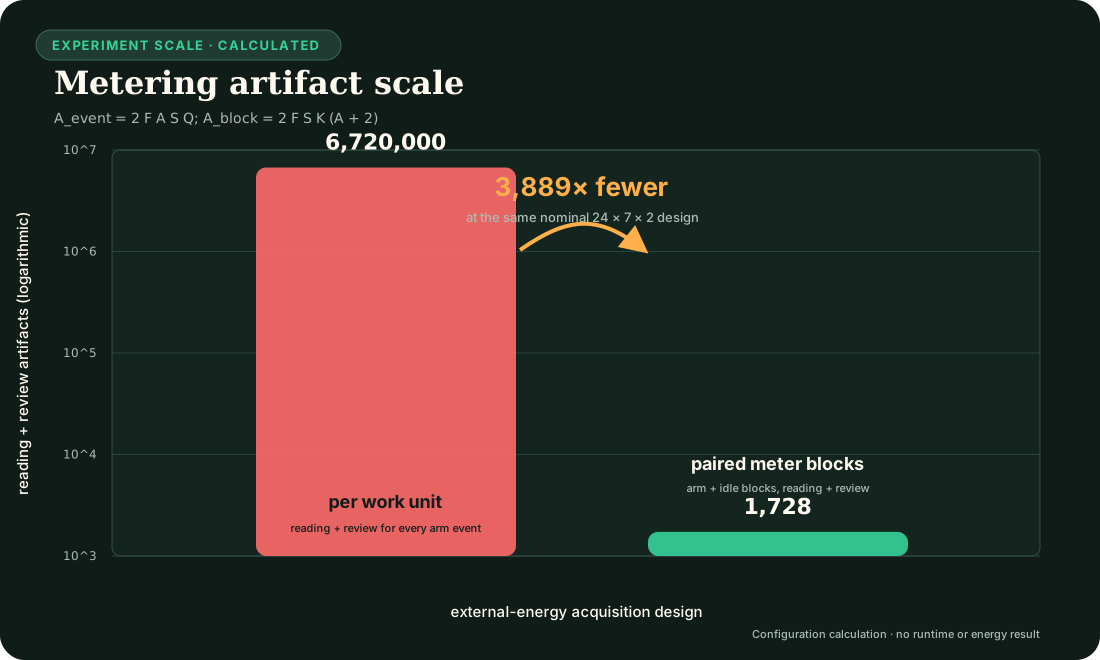
The nominal two-seed design would create 6,720,000 reading-plus-review files under per-work-unit metering but 1,728 under the current paired-block design. That is an artifact-count calculation, not an energy result or a larger sample size.
Editable assumptions:
../assets/plots/core-models.json.
Lifecycle energy
For candidate over horizon , define the disjoint lifecycle total
Every term is energy in joules at the same boundary :
- covers architecture search, hyperparameter tuning, and failed development runs attributable to the selected result;
- covers final training and validation;
- covers pruning, replay, merging, or structural stabilization before service;
- covers compilation, quantization, layout generation, and deployment preparation;
- covers event execution during ;
- covers monitoring, replay, repair, indexing, and lifecycle control during ;
- covers state serialization, transfer, warm-up, and reconfiguration not already assigned elsewhere;
- covers additional recovery work after a declared failure or regime change; and
- covers provisioned but inactive devices, memory, communication links, and reserve capacity during .
Fast control and slow structure therefore require separate action, build, carry, reversal, stranded-capacity, and recovery rows before any lifecycle advantage is claimed (C-1496).
An event is assigned to exactly one term. A migration byte, for example, may appear in the movement ledger but its energy is not also charged as ordinary serving traffic.
Protection is also a lifecycle state, not a free subtraction from damage. The electrochemical solid--electrolyte interphase is a useful accounting example: it can suppress an immediate parasitic reaction while consuming inventory, adding resistance, continuing to grow, and changing regime (C-1535). For an artificial barrier, define
with every term measured in joules at the same boundary. The result also keeps separate native-unit axes for consumed capacity, added latency, blocked useful work, false quarantine, damage admitted, and recovery. A filter, cache, trust layer, quarantine boundary, or checkpoint barrier wins only when its avoided downstream loss exceeds these construction, carrying, resistance, maintenance, and failure costs against fixed-barrier, rate-limiter, rollback, and no-barrier nulls. Cracking and repair in F-025 are synthetic engineering stressors, not effects attributed to the cited interphase sources.
Interface insulation uses the same lifecycle discipline but a different causal test. For an insulating path , retain separate energy rows for producing and copying snapshots, maintaining buffers or replicas, admission and expiry, monitoring connection sensitivity, serving consumers, recovery and idle reserve. Its accepted-service denominator must include timely and fresh consumer outputs; deleting, dropping or indefinitely delaying load cannot manufacture an energy saving. Logical operations and bytes are explanatory telemetry until a calibrated physical boundary measures joules (C-1555–C-1557).
No monotone insulation--energy law is assumed. One scoped biochemical model shows a fuel tradeoff, while a countermodel reduces both coupling and fuel by accepting worse tracking or leak robustness. The artificial comparison must therefore preserve the full distortion--service--latency--memory--work--energy frontier and the no-load case. The equations and decision boundary are in the interface-qualified retroactivity contract.
Delayed damage prevents short evaluations from closing that ledger. If is accumulated damage in a declared damage unit and is a state-, action-, temperature-, and mode-dependent damage rate in damage units per second, then
is dimensionally valid for step duration in seconds. Early outcome prediction may reduce the number of full-horizon trials, but reserve trials, false rankings, calendar exposure, and late failures remain charged (C-1539). A policy selected by a short proxy is not yet a lifecycle result.
Lifecycle energy per qualified event is
where is the candidate’s qualified-event count during and is joules/qualified event. The same result is also reported per offered event so quality filtering remains visible. Lower friction or wear at one coupon/contact cannot replace accepted system service, mission transfer, auxiliaries, maintenance, replacement, manufacture, or allocation uncertainty in this boundary (C-1505).
Break-even horizon
Let be candidate minus baseline one-time energy before service in joules, and let be the measured steady serving saving in joules/qualified event. When and , the event-count break-even point is
is a count. At qualified service rate in events/second, the time break-even is seconds. Maintenance, migration, recovery, and idle differences that grow with time must be included in the full numerical break-even calculation; the simple quotient is valid only when they are already represented in or are negligible over the stated horizon. A compiled surface or interface structure must include build, manufacture, inflexibility, reversal, and failed-envelope cost in this test (C-1503). If , there is no energy break-even.
Data movement ledger
Executed arithmetic and moved data remain separate observables. For one run,
where every term is bytes crossing the named, disjoint boundary: on-chip cache levels, device memory, host–device interface, inter-device or inter-node fabric, persistent storage, and migration path. The ledger additionally reports byte-hops, defined as payload bytes multiplied by traversed logical or physical links, in byte-hops. Reads and writes are separated when their costs differ.
Operation and movement counts can support a calibrated model,
where is the declared set of operation classes, is the executed count for class , is calibrated joules/operation, is the set of movement boundaries, is bytes crossing boundary , is calibrated joules/byte, and is modeled idle power in watts. A hat marks an estimate. The model is checked against gross measured energy; it never upgrades modeled joules into measured joules.
Numerical energy-per-operation tables are tied to process, device, precision, data locality, utilization, and year. The engineering audit therefore uses them as an accounting method, not constants (computer architecture analogue). The thermodynamic floor joules describes the minimum dissipation associated with erasing one bit under its physical assumptions; is the Boltzmann constant in joules/kelvin and is absolute temperature in kelvin. It is not an estimator for an inference, multiply, or memory transfer.
Relative sensing has a reference-maintenance ledger
A relative channel can appear cheaper by deleting amplitude-indexed parameters while silently importing a maintained reference. For reference state , the candidate ledger therefore separates
Each term is measured in joules only at a calibrated workstation boundary; before that, operations, writes, bytes and seconds remain separate. Channel- specific receptor abundance is biological evidence that a reference can be stored in interface structure (C-1548), not evidence that such storage is free. F-026 rejects the efficiency hypothesis if an explicit log ratio, streaming estimator, state-space model or compact recurrent state reaches the same task/risk frontier with lower complete maintenance cost.
Reduction and closure work stays inside the ledger
A coarse model is not credited with avoiding fine computation when its usable state depends on unreported reconstruction, healing, or fallback. For a multiscale run, define
where each term is gross measured electrical energy in joules attributable to lifting a coarse state, discarding initialization transients, advancing local fine simulations, restricting them back to coarse observables, coordinating micro/macro work, and executing a qualified fallback. The matching movement ledger separately reports bytes for every term; CPU seconds, solver steps, and right-hand-side evaluations remain non-energy diagnostics.
If a projected model truncates memory, the retained history window and omitted tail are part of the declared approximation (C-1526). If a slow reduction approaches a fold or loses its spectral gap, detection and fallback remain charged (C-1527). Heterogeneous micro-queries cannot receive free boundary reconstruction or synchronization (C-1528), and equation-free computation cannot hide lift replicas or healing inside preprocessing (C-1529). The complete dimensional and closure rules are in the multiscale-reduction contract.
The baseline receives an equally optimized implementation and the same error, risk, latency, and fallback envelope. A reduction wins only if its full measured lifecycle energy is lower after every failed query, rejected step, reconstruction, and coarse-model invalidation is retained.
Equal-budget comparisons
Candidate and baseline receive matched opportunity to succeed. Each experiment freezes:
- training and evaluation data, stream order, changes, failures, and seeds;
- quality, risk, latency, and availability requirements;
- input information and look-ahead—an oracle is labeled and never used as a superiority baseline;
- tuning trials and tuning compute in device-hours or joules;
- provisioned parameter, memory, module, edge, or replica capacity;
- service compute, controller compute, telemetry, and actuation cadence;
- migration, topology-edit, replay, and reserve ceilings;
- software optimization effort appropriate to both methods; and
- measurement boundary, duration, warm-up, repetitions, and instrumentation.
Some mechanisms intentionally exchange one resource for another. They are not forced into a single operation count; instead, all resource axes are recorded and the quality–risk–latency–energy–movement frontier is compared. A method that violates a hard budget is infeasible, not retroactively scaled into compliance.
Engineering null models
The relevant null model is the strongest standard solution to the same constrained problem, not only a dense network:
| Proposed mechanism | Minimum null model |
|---|---|
| Conditional routing | tuned dense reference, fixed sparse model, and budgeted adaptive router |
| Prediction-error compute | calibrated residual/change detector plus value-of-information acquisition |
| Homeostatic allocation | tuned feedback or primal/dual resource controller |
| Adaptive topology | fixed topology with adaptive weights/routing and periodic global graph optimization |
| Temporal communication | fixed optimized schedule and work-conserving scheduler |
| Memory tiers | tuned cache/TTL/retrieval policy and, where possible, an oracle-lifetime upper bound |
| Maintenance plane | periodic/adaptive checkpoint, monitoring, and recovery controller |
| Structural specialization | profile-guided compilation, layout, quantization, and accelerator-aware kernel |
| Connection-qualified insulation | immutable message or copy-on-write, bounded queue/backpressure, admission/expiry, resource isolation, explicit filter/controller, replication, and no-insulator control |
The full mapping and formal reference points are in the engineering analogue audit. Component ablations determine whether the claimed mechanism causes a gain. An oracle supplies headroom, while a shuffled or random-action control detects benefit from adaptation without useful information.
Evaluation loop
flowchart TB
    subgraph compare["1 · Freeze the comparison"]
        direction LR
        claim["Efficiency claim"] --> contract["Contract + strongest null"]
        contract --> paired["Matched paired trials"]
    end
    subgraph account["2 · Account for the lifecycle"]
        direction LR
        measure["Quality · energy · movement"] --> costs["Adaptation · recovery · uncertainty"]
    end
    subgraph decide["3 · Gate the result"]
        direction LR
        envelope{"Quality, risk, latency pass?"} --> gain{"Net gain over null?"}
        gain --> result["Promote, narrow, or reject"]
    end
    paired --> measure
    costs --> envelope
    result --> replicate["Replicate on another workload or hardware"]
Uncertainty and missing costs
The primary comparison is paired. Candidate and baseline run the same workload seed, event sequence, change schedule, and failure trace. For paired replicate , define relative lifecycle effect
where each is joules/qualified event and is dimensionless. Report the paired point estimate and a confidence interval across independent full-run seeds. Hierarchical bootstrap resampling is used when events are nested within seeds or change episodes. Repeated samples from one power trace are not treated as independent runs.
For a modeled scalar energy , where is the declared energy-model function and is its coefficient-and-count vector, local covariance propagation is
where is the vector of calibrated coefficients and measured counts, is their covariance matrix in the corresponding squared mixed units, and is the Jacobian row vector of partial derivatives of with respect to . The result is variance in joules squared. Bootstrap or Monte Carlo propagation replaces this approximation for nonlinear, correlated, or non-Gaussian estimates.
If a material category cannot yet be measured, let its energy lie in declared interval joules. The conclusion must survive the least favorable assignment within that interval. A result whose sign depends on assuming the missing category is zero remains unresolved.
Uncertainty reporting includes:
- meter accuracy, resolution, sampling rate, clock error, and calibration date;
- run-to-run variation, warm-up state, thermal state, and background workload;
- coefficient covariance and extrapolation range for modeled components;
- seed, task-stratum, failure, and change-event variation; and
- censored failures to finish or recover.
The uncertainty interval accompanies the effect and the absolute values. A large sample size does not repair a mismatched boundary or missing lifecycle phase.
Efficiency mechanism
The project’s mechanisms act on distinct terms of the lifecycle and movement ledger. They must earn their complexity against the appropriate null model.
| Lever | Intended physical change | Necessary measurements | Common null explanation |
|---|---|---|---|
| Selective modules and early exit | fewer executed operations and avoided activation movement | operation classes, device/host bytes, gate energy, latency by difficulty | tuned smaller dense model or confidence threshold matches it |
| Compartmentalization and placement | fewer cross-boundary bytes and smaller blast radius | byte-hops, cut traffic, placement/migration energy, recovery | ordinary partitioning or cache-aware layout matches it |
| Adaptive logical topology | fewer idle links and shorter useful paths under drift | edge-seconds, byte-hops, controller work, migration, reserve, recovery | adaptive weights or periodic graph optimization matches it |
| Memory lifetime routing | fewer expensive writes, replays, and stale retrievals | tier bytes, reads/writes, migration, retention quality, maintenance energy | LRU/TTL/retrieval policy matches it |
| Quantization and compilation | less arithmetic and movement per stable path | executed precision, kernel mix, bytes, compile energy, break-even | standard profile-guided optimization matches it |
| Maintenance and consolidation | lower future update/recovery cost after paid background work | replay/checkpoint bytes, optimizer work, downtime, retained quality, lifecycle horizon | periodic maintenance matches it |
| Temporal communication | less broadcast while meeting deadlines | physical context bytes, synchronization power, jitter, schedule-update cost | optimized time-aware schedule matches it |
The first candidate experiments instantiate the shared contract:
- adaptive topology prices edge updates, reserve, migration, and recovery against routing and graph-optimization baselines;
- multiscale context broadcast separates logical bandwidth from physical tensor movement and board energy; and
- recovery dynamics prices active probes, telemetry, latency, and false alarms against standard monitoring and system-identification baselines.
An operation saving becomes an energy mechanism only if it removes physical work at the chosen boundary. An arithmetic reduction that adds irregular dispatch, cache misses, synchronization, or migration may move cost rather than remove it.
Result hierarchy
Every experiment reports the narrowest supported level:
- Proxy reduction: fewer operations, bytes, active edges, or updates.
- Component reduction: lower measured energy at a named device or link.
- System reduction: lower gross node or cluster energy inside the matched quality, risk, and latency envelope.
- Lifecycle reduction: lower after search, adaptation, maintenance, reserve, failure, and idle costs at a declared horizon.
- Transfer: the lifecycle result replicates on another workload or hardware class without changing the claim after seeing the result.
Evidence at one level does not imply the next. This hierarchy makes a useful proxy result publishable without inflating it into an end-to-end claim.
Audit of the inherited comparison
The source discussion asserted that a 20-watt brain would correspond to hundreds of kilowatts or megawatts of accelerator power. The calculation mixed an assumed biological operation rate, peak accelerator arithmetic at varying precisions, and a facility multiplier. Its formal shape,
is dimensionally valid only when is brain power in watts, is machine power in watts, and both efficiencies measure the same qualified functional output per joule under the same quality, risk, time, and boundary record . No such common output has been established. The inherited values are retained as provenance for C-016, not as constants, bounds, or project targets.
The title “20 Watts Was Enough” expresses the research constraint: useful adaptive intelligence exists under a small biological power budget. The project’s numerical claims will come from the measurement loop above.
Evidence status
- Energy constrains biological signaling under the scoped evidence in C-001: established.
- Local sparse learning can be implemented on event-driven neuromorphic hardware under C-015: established for the cited systems, not proof of this architecture.
- The inherited biological-to-accelerator numerical range under C-016: disputed.
- Data movement, control, maintenance, and idle provision can dominate or erase nominal arithmetic savings: engineering null hypothesis to measure for each system, not a fixed proportion.
- Lower lifecycle energy from the integrated architecture at matched quality, risk, and latency: speculative until candidate experiments clear their preregistered gates and measured system boundaries.
Speculative extensions
Calibrated marginal-energy control
A controller could estimate the marginal joules of another layer, sensor, retrieval, replay, or route and compare it with expected decision improvement. The proxy would be trained from counters but recalibrated against gross energy measurements. Its calibration error and controller energy would be first-class outcomes.
Carbon- and scarcity-aware scheduling
Once joules are stable, execution time and placement could include marginal carbon intensity, water stress, or resource scarcity. These quantities retain their own units and uncertainty; they augment rather than replace the energy ledger.
Causal movement attribution
Hardware counters observe traffic but do not always identify which mechanism caused it. Controlled placement, cache-flush, route-freeze, and migration ablations could estimate the marginal bytes and joules caused by a gate, memory tier, or topology update.
Cross-substrate transfer model
A hierarchy of calibrated energy models could predict which mechanisms retain their advantage across GPUs, CPUs, accelerators, and distributed nodes. The transfer model would predict the sign and break-even horizon before the new hardware run, then be scored on calibration rather than refit after every result.
Failure modes
- Boundary drift: device energy is described as node, cluster, or facility energy without measuring the added components.
- Quality leakage: the candidate saves energy by rejecting hard inputs, lowering rare-event quality, or exceeding the latency envelope.
- Weak null model: a new controller is compared only with dense execution when tuned routing, caching, control, scheduling, or compilation solves the same problem.
- Unpriced adaptation: search, telemetry, replay, state movement, reserve, rollback, and failed updates disappear from the ledger.
- Double counting: migration or maintenance energy appears in both serving traffic and its own lifecycle category.
- Proxy substitution: FLOPs, parameters, active modules, logical messages, TDP, peak throughput, or a vendor operation table is reported as measured energy.
- Idle erasure: baseline subtraction removes capacity that the candidate must keep powered for latency or recovery.
- Amortization without demand: a one-time optimization is divided by an assumed event count beyond the measured deployment horizon.
- Uncertainty collapse: samples within one power trace are treated as independent replicates, or missing components are assigned zero uncertainty.
- Optimization asymmetry: the candidate receives more tuning trials, future information, custom kernels, or favorable batch/precision settings.
- Hardware overgeneralization: an irregular sparse win or loss on one substrate is stated as an architecture-wide property.
- Thermodynamic rhetoric: the Landauer floor or a 20-watt biological value is used to estimate attainable contemporary system energy.
Measurable predictions
H-E1 — Conditional execution
At matched quality, risk, and latency, a conditional path will reduce gross node joules/qualified event only after avoided module compute and physical data movement exceed gating, dispatch, and lost-utilization overhead. A tuned smaller dense model and fixed sparse model are required nulls. Reject the mechanism-level energy claim if the saving exists only in operation counts.
H-E2 — Data movement
Placement, compartmentalization, and structural consolidation will reduce host–device and inter-device byte/qualified event as well as byte-hops. The effect should predict a measured energy reduction after calibration. Reject the placement explanation if bytes do not fall or an ordinary partition/layout baseline matches it.
H-E3 — Lifecycle break-even
Pruning, compilation, consolidation, or specialization will have a finite and inside the measured deployment horizon. The result must remain positive after search, failed runs, maintenance, and rollback are included. Report “no break-even” when steady serving savings are non-positive or the observed horizon ends first.
H-E4 — Adaptive topology
Under recurrent changes and faults, use-dependent topology will reduce full lifecycle modeled and then measured joules/timely utility unit without violating quality or recovery margins. It must beat fixed topology with adaptive routing and budget-matched periodic graph optimization, and its frozen-topology ablation must lose the advantage. The Stage-1 thresholds are defined in Candidate 001.
H-E5 — Memory lifecycle
Lifetime-aware memory actions will reduce replay, write, retrieval, and migration energy at a declared retention and obsolete-intrusion envelope. A tuned cache/TTL/retrieval policy is the null. The scheduling and provenance overhead must be included in the break-even horizon described by the memory-lifecycle model.
H-E6 — Recovery-aware efficiency
A system with lower normal-operation energy but materially slower or less reliable recovery will not dominate. Energy, utility deficit in utility-seconds, and recovery time in seconds are reported jointly under paired faults and regime changes. Reserve capacity is charged in watt-seconds even when unused.
H-E7 — Substrate transfer
A mechanism promoted beyond one device will retain the direction of lifecycle effect on at least one second hardware class using the same task envelope and an independently calibrated movement model. If the sign changes, the result is reported as substrate-specific and the counters responsible for the reversal must be identified.
The project advances an efficiency claim only when the strongest engineering null model is outside the preregistered equivalence margin and the full lifecycle confidence interval clears the material-effect threshold. Otherwise the result narrows the design space and the biological principle remains a source of hypotheses rather than a performance claim.