Interface-qualified scale symmetry — 20 Watts Was Enough

lusoris contributors

Purpose: define and visualize full-trajectory fold-change detection, weaker lookalikes, observation-interface dependence, and the cost of preserving an absolute side channel
Claims: C-1540--C-1549
Evidence audit: relative sensing and scale symmetry
Experiment contract: Fixture F-026
Result state: analytical definitions and one illustrative exact model; no trained-model, biological, workstation or energy result

Notation, units, and interfaces

Symbol	Meaning	Unit
$t$	time	seconds (s)
$x(t)$	internal state vector	model-declared
$u(t)$	positive external input	model-declared input unit
$b$	positive background input	same unit as $u$
$p$	positive multiplicative scale factor	dimensionless
$G$	registered set of admissible scale factors	dimensionless set
$y(t)$	output at one declared interface	model-declared
$r(t)$	positive reference state	same unit as $u$
$\tau_r$	reference time constant	seconds (s)
$m$	pulse fold multiplier	dimensionless
$D_{j,p}$	normalized trajectory discrepancy	dimensionless
$s_{y,j}$	frozen nonzero scale for output component $j$	same unit as $y_j$

The observation chain is

u_{\mathrm{external}} \longrightarrow u_{\mathrm{internal}} \longrightarrow y_{\mathrm{readout}} \longrightarrow a_{\mathrm{action}}.

Scale symmetry at one arrow does not imply it at the next. The input, state, readout, target and action must therefore be named independently.

Exact full-trajectory definition

Consider a causal system

\dot{x}=f(x,u), \qquad y=h(x,u),

and let $x_{\mathrm{ss}}(b)$ be the initialized steady state associated with positive background $b$ . Exact FCD over scale support $G$ requires

y\!\left(t; p u, x_{\mathrm{ss}}(pb)\right) = y\!\left(t; u, x_{\mathrm{ss}}(b)\right)

for every registered input history, time, and $p\in G$ . The equality is between complete trajectories. Equality of a final value, peak, integral or selected time point is insufficient.

Approximate FCD needs a frozen discrepancy, support, uncertainty model and acceptance margin. It is not licensed by a visually attractive overlay.

State-equivariance certificate

Assume the model has unique solutions on a declared forward-invariant positive domain, and that $\rho_p$ maps that domain into itself for every $p\in G$ . Let $\rho_p$ transform internal state when the positive input is multiplied by $p$ . Under those conditions, a sufficient certificate is

f\!\left(\rho_p(x),pu\right) = D\rho_p(x)f(x,u),

h\!\left(\rho_p(x),pu\right) = h(x,u),

and

\rho_p\!\left(x_{\mathrm{ss}}(b)\right) = x_{\mathrm{ss}}(pb).

$D\rho_p(x)$ is the Jacobian of the state transformation. These equalities belong to a defined model and observation map. Changing the output can change both invariance and identifiability.

Worked reference model

Use the positive-domain reference system

\tau_r\dot r=u-r, \qquad y=\ln\frac{u}{r}.

Under the transformation $(u,r)\mapsto(pu,pr)$ , the state equation scales by $p$ while the output remains

\ln\frac{pu}{pr}=\ln\frac{u}{r}.

If $r(0)=b$ , then the transformed initial state is $pr(0)=pb$ , so the entire output trajectory is identical.

For a pulse that changes $u$ from $b$ to $mb$ at $t_0$ and returns to $b$ at $t_1$ , the reference during the pulse is

r(t) = b\left[m-(m-1)e^{-(t-t_0)/\tau_r}\right], \qquad t_0\le t<t_1,

and the relative output is

y(t) = \ln\frac{m}{m-(m-1)e^{-(t-t_0)/\tau_r}}.

The background $b$ cancels. After the pulse, define

q = (m-1)\left(1-e^{-(t_1-t_0)/\tau_r}\right).

Then

r(t)=b\left[1+q e^{-(t-t_1)/\tau_r}\right], \qquad y(t)=-\ln\left[1+q e^{-(t-t_1)/\tau_r}\right],

which is again independent of $b$ .

Two geometrically scaled input/reference paths follow the same ratio contours and produce identical relative trajectories, while a separate absolute gate distinguishes them.

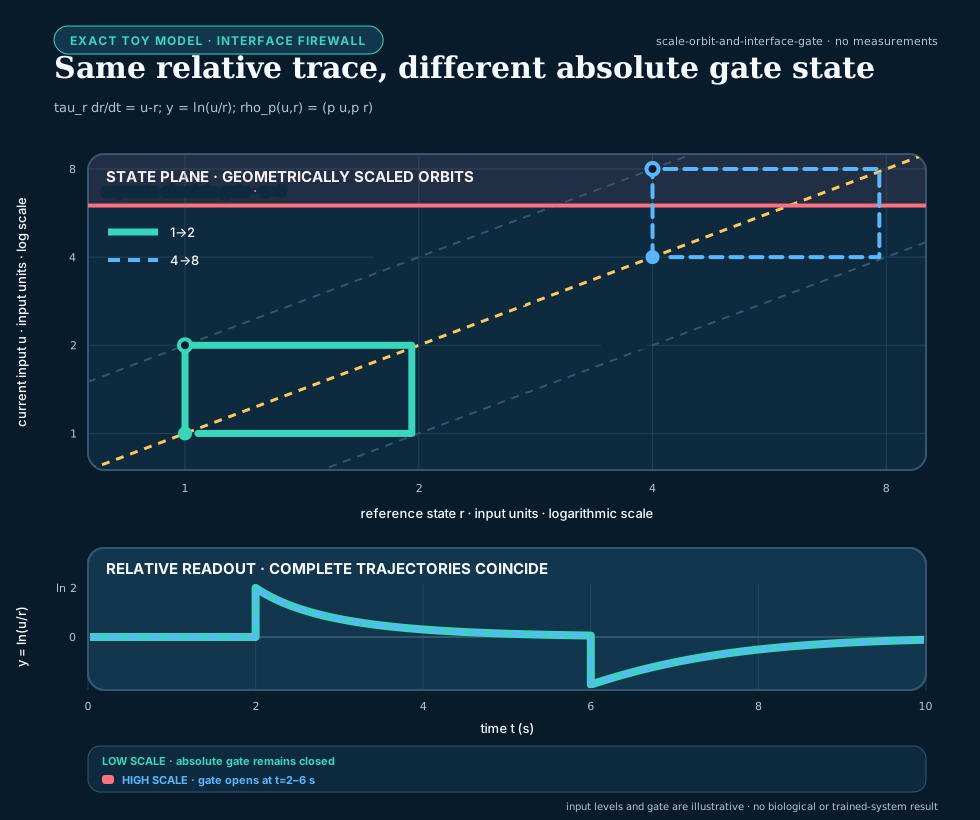
The figure uses $b\in\{1,4\}$ , $m=2$ , $\tau_r=1.25\,\mathrm{s}$ and an illustrative absolute gate at $u=6$ input units. The relative traces coincide exactly in this model, but the $4\rightarrow8$ pulse crosses the gate while the $1\rightarrow2$ pulse does not. The gate is a mathematical counter-task, not a biological or safety threshold.

Weaker lookalikes

The constructions below are properties, not disjoint mechanism classes. A static ratio map with its reference supplied at the interface can satisfy exact trajectory symmetry, and endpoint return can coexist with equal peak. F-026 therefore keeps generator family as secondary provenance and evaluates cross-cutting properties separately while retaining their logical dependencies.

Finite-horizon endpoint return

A finite recorded trajectory can test return relative to each trajectory's own prestimulus output. On a frozen discrete horizon with endpoint tolerance $\varepsilon_{\mathrm{end}}$ , define

A_{\mathrm{end},j,h,p} = \mathbb{1}\!\left[ |y_{j,h,1,N}-y_{j,h,1,0}|\le\varepsilon_{\mathrm{end}} \;\land\; |y_{j,h,p,N}-y_{j,h,p,0}|\le\varepsilon_{\mathrm{end}} \right].

This finite-sample predicate is not general exact adaptation. A pulse can return because the input itself returned, and one forced final sample says nothing about causality or settling. Exact adaptation instead requires a declared sustained-input equilibrium or registered settling-tail condition; in the ideal infinite-horizon form,

\lim_{t\rightarrow\infty}y(t)=y_0.

Two systems can share $y_0$ while their peak, latency, width and tail differ.

Weber-like peak equality

Peak equality is measured as maximum absolute departure from each trajectory's own prestimulus value,

P_{j,h,p}=\max_k |y_{j,h,p,k}-y_{j,h,p,0}|, \qquad P_{j,h,1}=\max_k |y_{j,h,1,k}-y_{j,h,1,0}|.

The first maximizing sample is the frozen latency tie-break. Equality of $P_{j,h,p}$ and $P_{j,h,1}$ does not constrain latency or the rest of the trajectory.

Static normalization

A static value $u_t/r_t$ has no necessary causal rule for producing, aging, validating or resetting $r_t$ . Its output can look relative while its reference uses future data or stale support.

Additive difference and derivative

For positive $u$ and a frozen positive reference unit $u_*$ with the same input unit,

\ln\frac{u(t)}{u_*}-\ln\frac{b}{u_*} =\ln\frac{u(t)}{b}

is invariant to a common multiplicative scale. In contrast, $u(t)-b$ is invariant to a common additive offset, and $du/dt$ responds to a rate in input units per second. Limited step or ramp families can confound these statistics.

Approximate trajectory score

For output component $j$ , registered input history $h\in\mathcal H$ , held-out factor $p\in\mathcal P$ , duration $T$ seconds and frozen nonzero scale $s_{y,j}$ , use

D_{j,h,p} = \sqrt{ \frac{1}{T} \int_0^T \left\| \frac{y_{j,h,p}(t)-y_{j,h,1}(t)}{s_{y,j}} \right\|^2dt }.

The score is dimensionless. The scale $s_{y,j}$ , integration grid, time window, scale factors and uncertainty procedure must be frozen before confirmation. Report peak, latency, duration and tail discrepancies separately so a low integral error cannot hide one dangerous phase.

System-level classification uses the worst registered cell, not an unstated average:

D_{j,\max}=\max_{h\in\mathcal H,\,p\in\mathcal P}D_{j,h,p}.

With frozen tolerances $0\le\varepsilon_{\mathrm{exact}}<\varepsilon_{\mathrm{approx}}$ , define the tolerance-qualified class

S_{\mathrm{system},j}= \begin{cases} \mathrm{exact}, & D_{j,\max}\le\varepsilon_{\mathrm{exact}},\\ \mathrm{approximate}, & \varepsilon_{\mathrm{exact}}<D_{j,\max} \le\varepsilon_{\mathrm{approx}},\\ \mathrm{absent}, & D_{j,\max}>\varepsilon_{\mathrm{approx}}. \end{cases}

Missing or rejected cells do not disappear from the maximum; they make the system classification unavailable and retain an abstention in its registered denominator.

If an actionable arm receives both complete output trajectories on this grid, $D_{j,h,p}$ , paired trajectory match, finite-horizon endpoint return and peak equality are directly computable. Their errors measure numerical conformance and the resource cost of producing the values; they are not evidence that a representation learned the properties. A predictive interpretation needs a separately registered prospective observation cut, such as a withheld suffix, scale cell, or future intervention. That cut must state what the arm observes, what remains evaluator-only, and when its response freezes. Merely labelling a publicly enumerated scale as “withheld” does not create confirmatory secrecy.

The RSD-T01 development foundation therefore separates three objects:

a complete history × scale descriptor grid, including multiple scale cells per shared initialization and a predeclared prospective role;
valid scientific hostile worlds with explicit support membership and expected leakage behavior; and
malformed-record sentinels, which test fail-closed parsing and never enter the scientific denominator.

Its dimensionless scale sets are

\mathcal P_{\mathrm{development}}=\{2,4\}, \qquad \mathcal P_{\mathrm{prospective}}=\{8\}, \qquad \mathcal P=\mathcal P_{\mathrm{development}} \cup\mathcal P_{\mathrm{prospective}}.

Every $p\in\mathcal P$ multiplies the same $p=1$ reference trajectory and shares the registered initialization identity. “Prospective” is a public descriptor role here, not a concealed confirmation partition.

This descriptor foundation can test grid construction and aggregation while the predictive observation cut remains blocked. It has no comparator-result or claim authority.

For the current RSD-T01 contract the evaluator's property target is

\boldsymbol\pi_j= \left( S_{\mathrm{system},j}, \{A_{\mathrm{end},j,h,p}\}_{h,p}, \{E_{\mathrm{peak},j,h,p}\}_{h,p}, M_{\mathrm{causal}}, \mathbf Q_{\mathrm{membership},j} \right),

where $S_{\mathrm{system},j}\in\{\mathrm{exact},\mathrm{approximate},\mathrm{absent}\}$ is evaluated by $D_{j,\max}$ across the complete frozen history × scale grid rather than inferred from one pair, $A_{\mathrm{end},j,h,p}$ is the per-cell finite-horizon endpoint predicate, $E_{\mathrm{peak},j,h,p}$ is the per-cell tolerance-qualified equality of $P_{j,h,p}$ and $P_{j,h,1}$ , $M_{\mathrm{causal}}$ requires a machine-readable state equation or identifying intervention, and $\mathbf Q_{\mathrm{membership},j}$ is generator truth with one $\{\mathrm{inside},\mathrm{outside}\}$ coordinate for each registered support axis: input domain, transformation family, instrument range, initialization contract, causal observation contract, and evaluation window. This vector prevents an additive transformation, clipped measurement, hidden reset, or future-aware normalizer from being collapsed into one ambiguous bit. An arm's support-detection decision is a separate output because detectability depends on its observation interface. The endpoint and peak matrices remain primary data. A compact summary may use only the frozen reducer all when every registered cell is true, none when every cell is false, and partial otherwise; it may not silently substitute a mean. These coordinates are asserted without using the generator-family name, but they are not logically independent: exact trajectory equality, for example, implies equal peak under the same peak definition.

The public generator-only smoke layer records a narrower per-world vector: paired-trajectory match, finite-horizon endpoint return, peak-amplitude equality, causal_memory_status: unassessed, and support_membership: inside. It does not promote one paired trace to a system symmetry certificate. That legacy scalar is a narrower v2 smoke field; it does not replace the axis-qualified vector in the scientific-grid foundation.

Property vector, not family label

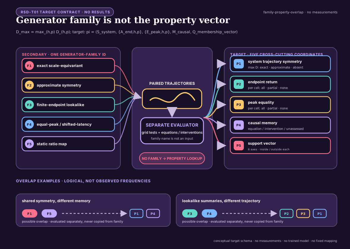
Five generator-family labels converge through paired trajectories into a separate evaluator, which produces five cross-cutting property coordinates while retaining logical dependencies; two examples show that different families can share properties while differing on others.

The family ID remains a secondary synthetic diagnostic. The primary vector is evaluated from the registered trajectory grid, structural equations and interventions; it is never copied from a family-to-property lookup. The current smoke records only its directly observable subset and marks causal memory unassessed. The editable figure specification is the rsd-t01-family-property-overlap entry in core-models.json.

RSD-T02 uses the same rule at a deeper causal level. Its dedicated intervention-qualified mechanism-equivalence note constructs five exact matched-step recipes, scores separately certified structural properties and retains observational equivalence or abstention. It also keeps the Skataric--Nikolaev--Sontag fast-boundary-layer endpoint separate from the RMS score above: the source-qualified floor is a supremum-norm result on an $\epsilon$ -scaled temporal grid, while an integrated RMS discrepancy can vanish as the layer narrows.

Validity and failure boundaries

Positive support. Log ratio is undefined at zero and changes meaning across sign. A hidden epsilon is not a scientific solution.
Saturation and clipping. Multiplicative histories can become observationally identical for the wrong reason.
Additive shift. A ratio-qualified model need not transfer across added backgrounds.
Reference age. A stale or contaminated $r_t$ changes the statistic even when the current $u_t$ is valid.
Initialization. Comparing trajectories from unmatched states does not test the stated symmetry.
Protocol support. Steps alone do not certify pulses, ramps, stochastic histories or closed-loop action.
Interface. Relative encoding upstream can become absolute or difference-based downstream.
Absolute target. If the target depends on $u$ rather than $u/r$ , a relative-only representation is insufficient by construction.

Observation and recoverability

If an output is exactly invariant under a transformation, that transformed quantity can be structurally unidentifiable from that output interface under the declared initialized model. This is an observation-qualified statement, not universal destruction of information. Recoverability can change when one adds an output, fixes a parameter, changes initialization, or supplies a calibrated absolute observation.

F-026 therefore reports three axes separately:

robustness to nuisance multiplicative scale;
recoverability of every protected absolute quantity; and
complete observation, state, compute and maintenance cost.

Resource model

The authoritative report is a typed vector, not a sum of unlike units:

\mathbf q= \left( L_{\mathrm{task}}, \mathbf r_{\mathrm{risk}}, N_{\mathrm{op}}, B_{\mathrm{comm}}, B_{\mathrm{state}}, T_{\mathrm{wall}}, E_{\mathrm{ws}}, N_{\mathrm{ref}} \right).

Here $L_{\mathrm{task}}$ retains its task-native unit; $\mathbf r_{\mathrm{risk}}$ retains one registered unit per risk component; $N_{\mathrm{op}}$ and $N_{\mathrm{ref}}$ are operation and reference-lifecycle counts; $B_{\mathrm{comm}}$ and $B_{\mathrm{state}}$ are bytes; $T_{\mathrm{wall}}$ is seconds; and measured workstation energy $E_{\mathrm{ws}}$ is joules. None is inferred from another.

If a frozen decision rule genuinely needs a scalar diagnostic, every component requires its own conversion weight into one declared decision unit:

J= \lambda_L L_{\mathrm{task}} +\boldsymbol{\lambda}_r^{\mathsf T}\mathbf r_{\mathrm{risk}} +\lambda_N N_{\mathrm{op}} +\lambda_{Bc}B_{\mathrm{comm}} +\lambda_{Bs}B_{\mathrm{state}} +\lambda_TT_{\mathrm{wall}} +\lambda_EE_{\mathrm{ws}} +\lambda_U N_{\mathrm{ref}}.

Reference updates, calibration, resets, selector execution, abstention, fallback, writes and artifacts must appear in the appropriate count, byte and time components. A biological FCD paper does not supply any of these AI conversion weights.

Test and retirement conditions

The relative translation remains viable only if it:

lowers held-out task loss or complete work against static, streaming, log-ratio, state-space and recurrent nulls;
preserves every absolute-critical counter-task or abstains before action;
survives non-step multiplicative histories inside declared support;
rejects additive, near-zero, saturated and stale-reference cases; and
retains its advantage after reference maintenance and fallback are charged.

Retire the translation if a simpler explicit transform or ordinary estimator matches it, if full-trajectory invariance collapses to peak equality, or if a calibrated absolute channel recreates the cost of keeping raw state everywhere.