- Purpose: freeze the equations, property ontology, intervention interface, abstention rule and singular-boundary-layer metric for RSD-T02
- Claims: C-1541 and C-1560, C-1561, C-1562, C-1563, C-1564, C-1565, C-1566, C-1567, and C-1568
- Evidence audits: mechanism equivalence and intervention-qualified discrimination · population, identifiability, calibration, and null maturity
- Decisions: 0019 — score interventional properties, not generator names · 0020 — separate information cuts from scientific replication · 0021 — bind population inference to system lineages and instances
- Experiment contract: Fixture F-026, RSD-T02
- Result state: public-development equation and contract foundation;
NO_RESULT, no implemented estimator comparison, no confirmation custody and no energy measurement
Two different questions
RSD-T02 contains two linked but mathematically different strata:
T02-MECHasks which structural or interventional properties can be distinguished after several synthetic systems are forced to have the same canonical step response.T02-FLOORasks whether an estimator recovers a source-qualified supremum-norm error floor in a singularly perturbed system.
The first is a model-discrimination problem. The second is a norm and temporal resolution problem. Combining them into one family label or one integrated trajectory score would make both endpoints ambiguous.
Notation and units
| Symbol | Meaning | Unit |
|---|---|---|
| physical time | seconds (s) | |
| input on channel | input unit (U) | |
| registered positive background | U | |
| background-normalized input | dimensionless | |
| canonical fold, fixed to | dimensionless | |
| matched response time constant | s | |
| internal states | dimensionless | |
| internal output before a registered clamp | dimensionless | |
| reported output | dimensionless | |
| registered intervention panel | finite set | |
| maximum output difference between recipes under intervention | dimensionless | |
| RMS output difference | dimensionless | |
| fast/slow time-scale ratio | dimensionless | |
| positive multiplicative scale factor | dimensionless | |
| maximum instantaneous FCD discrepancy | dimensionless | |
| integrated RMS discrepancy | dimensionless |
The synthetic T02 input support uses , , and strictly positive normalized input. These are frozen benchmark design values, not biological estimates.
Exact matched-step construction
Every mechanism recipe starts at the steady normalized background and receives the canonical step . All five recipes must produce
This removes ordinary step fit as a discriminator by construction. The generator recipe remains evaluator-only provenance.
Input-driven incoherent feed-forward recipe
Use
The direct path and delayed antagonistic path form the operational feed-forward structure. For a constant post-step input ,
and therefore .
This is a synthetic reduced recipe inspired by the functional structure. It is not asserted to be the molecular equation set of a particular organism.
Nonlinear output-feedback recipe
Let
Normally . During the registered output-clamp intervention, is forced inside the feedback edge while remains evaluator-visible after response freeze. The nonlinear term is zero at both and . On the canonical step,
which gives the same . Away from that step and under the output clamp, the state update differs.
Channel-local receptor/reference memory
For , use
only for the active channel. The inactive channel retains its own reference. The first active-channel step again yields , while same-channel and cross-channel restimulation test state locality.
Static normalization plus an ordinary high-pass readout
Define the static affine fold transform
followed by
The normalization reference is static, but the complete system is not memoryless: the ordinary high-pass filter has causal state. On the canonical step , so and .
This recipe is input--output isomorphic to the reduced I1-FFL recipe under the registered affine interface. Their names must not be forced apart.
Explicit log difference plus the same readout order
For , define
The canonical step again has . Other folds and ramps distinguish the log transform from the affine transform. Nonpositive input is outside support and forces abstention; no hidden numerical epsilon is inserted.
Matched-step certificate
For recipes and , background , time constant and output samples , define
A public-development pack is invalid unless:
- every initialization residual is at most ;
- every registered recipe pair has ;
- the canonical step policy projection contains no recipe, equation, state, parameter or property identifier; and
- every actionable arm receives the same projection hash.
The tolerances are benchmark design constants. They are not empirical biological margins and grant no result authority.
Property vector and equivalence
The primary target is the evaluator-certified vector
where:
- ;
- states whether the reported output participates in a state-update feedback edge;
- states whether reference state is channel-local;
- is certified from equations or an identifying intervention, never from a finite trace alone.
Nonlinear update form remains equation provenance in the v1 bank. It perfectly co-varies with the output-feedback coordinate across these five worlds, so the contract cannot honestly score it as a separately identified property without adding a counterworld that breaks that dependence.
For intervention panel , observation map , sample grid and initialized recipes , define
A pair with different property vectors is numerically separated only when one frozen intervention has estimate and numerical error bound satisfying
An analytic equivalence or a complete bounded finite-grid equivalence with may retain both recipes. A claimed analytic equivalence that conflicts with its numerical bound is invalid rather than silently unresolved. Every other case is unresolved.
The I1-FFL and affine high-pass recipes deliberately share one operational property vector and one full-panel equivalence class. Guessing between their hidden names is an error, not added accuracy.
The v1 construction certificates are scoped to , , a horizon, 64 output samples per second and binary64 RK4. Discontinuous commands use half-open intervals and the left limit for the final RK4 stage ending on an event; the next step starts from the right-limit command. Distances at internal steps and must differ by at most . The conservative construction lower bounds are for the clamp and cross-channel certificates and for the affine-versus-log ramp certificate. These margin checks reproduce a synthetic construction; they are not empirical mechanism evidence or confirmation results.
Nested intervention panels
The full fixed panel contains exactly 26 episodes:
- three canonical steps at the three backgrounds;
- six repeated-pulse cells obtained from and with ;
- eight ramps: linear or exponential, up or down, each lasting or ;
- two opaque-state resets;
- two opaque-state freezes;
- one reported-output clamp;
- two interrupted-ramp holds lasting or ; and
- same-channel and cross-channel restimulation.
Every episode lasts . The noncanonical episodes use and . Periodic pulses have on while that interval remains inside the episode and otherwise. For ramp duration , let . Linear-in-fold ramps use
and linear-in-log-fold ramps use
with for up-ramps and for down-ramps. Reset occurs at ; state freezes and the reported-output clamp occupy . Interrupted ramps pause after one second of active ramp progress and resume after the registered hold. Restimulation drives channel A on , returns both channels to one on , then drives A or B on . The machine contract carries these numbers in each episode descriptor.
Every recipe exposes two opaque handles. A single-state recipe receives an inert padding state, and a seed-derived hidden permutation maps states to handles. State count and semantic node names therefore do not identify the recipe.
The observation regimes are:
O0-MATCHED-STEP: three background episodes and at most 4,611 sample rows per conditioned model instance. The construction runtime crosses , so each recipe has nine executions and 13,833 rows; every varying structural coordinate requires abstention.O1-FULL-PANEL: all 26 episodes and at most 39,962 sample rows at the fixed construction scope; this is the full-panel regime.O2-SELECT6: the three step episodes plus at most six selected queries, no more than two privileged internal queries, and at most 13,833 sample rows; it is a secondary active-design regime.
The current code freezes these regimes and analytic construction certificates. An additive whole-system Stage 2 now implements all nine registered public-development policy-conformance references. These fixed policies close the executable feature-family matrix; they do not constitute trained estimators, calibrated posteriors, mature nulls, a claim-eligible run or a comparison.
Fixed whole-system policy-conformance references
Let the ordered packet be with 53,795 sample rows.
All nine active policies receive the same canonical bytes and common cap. Their
responses are committed before O-GRAPH opens any member of . The bands
below were chosen after inspecting the five enumerated public construction
worlds. They are therefore construction-tuned protocol constants, not
fitted parameters or confirmation-calibrated decision limits.
Each packet is evaluated in a fresh Node child and one new hardened VM context.
The self-contained bank evaluates the nine ordered policies in that context.
The child receives one canonical LF JSON request and can read only the verified
SHA-named policy bundle. The policy VM receives no
process, filesystem, network, environment, clock, random or evaluator
capability.
Request, packet, configuration, bundle and runtime identities are bound into
the returned receipt. Time, memory, request, stdout and stderr are capped, and
any timeout, crash, malformed frame, replay or work-envelope violation becomes
an ordered pre-evaluator abstention with no retry or same-process fallback. The
runner atomically persists that outcome as a self-hashed
rsd-t02-arm-abstention.json, replay-binds it on later invocations and forbids
it from coexisting with the commitment or evaluator ledger.
Commitment creation remains exclusive and file-synchronized before the raw
evaluator ledger opens. The generator and evaluator are still statically
loaded before their later file fingerprints, so concurrent repository mutation
across that parent-module load boundary remains outside this
public-development authority; the policy computation itself executes from the
verified content-addressed bundle.
The six transform-policy references added in Stage 2b are deliberately small and causal. Let be the reported output, the active-channel input, the same-episode initial background, , and .
A-RAW uses no engineered drive coordinate. It reads the intervention traces
directly:
and uses the reset/freeze distance defined below. It declares a feedback edge for , no edge for , local channel state for , shared state for , memory for , and no memory for . It always abstains on the drive transform.
B-STATIC-DIV evaluates the ramp at using
It declares log-fold for , affine-fold for , and
otherwise abstains. B-LOG-RATIO instead uses the positive-domain coordinate
declaring log-fold for , affine-fold for , and abstaining when the logarithm is undefined or the evidence lies in the gap.
B-DIFFERENCE uses only the first 64 ramp increments. With
and
, its projection coefficient is
It declares affine-fold for , log-fold for , and otherwise abstains.
B-STREAM processes each selected trace in chronological order. For
, it updates
and scores the causal standardized innovation . Clamp-release evidence at one second uses true/false thresholds ; cross-channel restimulation at two seconds uses . Intermediate evidence abstains.
C-DUAL requires all three drive votes from , , and to be
present and identical. It then carries the supported raw intervention
decisions for the other three coordinates. Missing or discordant drive votes
produce an abstention; the frozen fallback count is zero.
For B-STATE-SPACE, define the fold and two fixed drives
For each drive, the reference recursion and one-step reported-output residual are
With , the margin declares affine for , log for , and otherwise abstains. Its memory signature is
It declares memory present for , absent for , and otherwise abstains. Feedback-edge and channel-local coordinates are always outside this reference's bounded scope.
For B-RECURRENT, the causal state update is
The absolute innovation at reported-output clamp release declares a feedback edge for values at least , no edge for values at most , and otherwise abstains. A separate state per observed channel gives the cross-channel restimulation innovation; values at least declare local state, values at most declare shared state, and intermediate values abstain. Drive and causal-memory coordinates remain outside this reference's scope.
C-MECHANISM-BANK uses four direct, frozen source-shaped signatures: linear
up-ramp output at (log at least , affine at most
), absolute clamp-release output (feedback at least , absent at
most ), maximum absolute cross-restimulation output on
(local at least , shared at most ), and above (memory at least
, absent at most ). Every indifference band forces abstention.
The five candidate equation identities and their bytes are charged separately
from the four distinct joint property-prior vectors and their bytes.
The semantic output is the joint set
with duplicate vectors removed but their compatible hypothesis IDs retained. must be nonempty, and every declared marginal must agree with every member of . This prevents independently plausible marginals from forming an impossible property combination.
Resource accounting is three-part: (1) shared acquisition of 35 episodes,
53,795 rows, 197 input commands, two resets, two freezes, one output clamp, one
channel switch and two state writes; (2) policy construction/prior artifacts,
threshold provenance, equations, vectors, labels and tuning; and (3) actual
per-inference work. Every policy is charged 12 declared traversal operations
per row, or 645,540 before its specific operations. Common caps are
scalar operations, 2,000 transcendental evaluations, 128 retained-state bytes,
4,096 influential-parameter bytes, 16 MiB scratch, 256 KiB combined policy and
configuration artifacts, and zero fallbacks. Actual counts are not padded to
the caps. Across the nine references, charged scalar work ranges from 645,544
(B-STATIC-DIV and B-LOG-RATIO) to 688,576 (B-STATE-SPACE), including the
common packet traversal. Wall time and joules remain null.
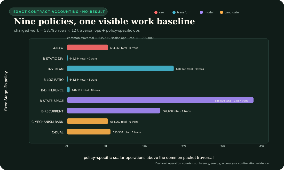
The plot exposes the common charge and the remaining policy-specific work without turning the declared scalar-operation model into a wall-time, energy or architecture-ranking claim.
The repeated-pulse grid is retained because the Rahi evidence makes refractory stabilization and period skipping useful one-sided signatures in a different bounded model class. The current five-world bank does not instantiate that signature: its registered feedback nonlinearity is zero at both square- pulse levels. C-1561 is specified separately in the repeated-stimulus topology-signature contract; it is not a claim supported by these five-world construction tests.
Prospective fit, calibration and evaluation cut
The Stage-3 design partitions the ordered 64-seed public pack once: ordered
positions 1--32 are fit, 33--48 are calibration, and 49--64 are
evaluation. The literal seed labels remain the frozen values
1540001--1540064; the position numbers are not substitute seeds.
Parameters and fit-only model selection stop at the first boundary;
probability calibration plus support and abstention thresholds stop at the
second; evaluation is one-pass frozen inference and scoring. Every future
artifact must bind the preceding artifact and the exact partition identity.
That split controls access, not replication. In the present generator, a seed
selects one of only two hidden permutations of two opaque state handles. The
permutation can swap which internal coordinate a reset or freeze targets, but
it does not sample a new equation, parameter set, input history or noisy
system. The 64 labels therefore cannot be analyzed as 64 independent systems,
and the public split has no comparison or power authority.
This is the scoped experimental-unit problem described by
Hurlbert (1984), bibliography key
hurlbert1984pseudoreplication, not a statement
that seeds can never be valid units in other generators.
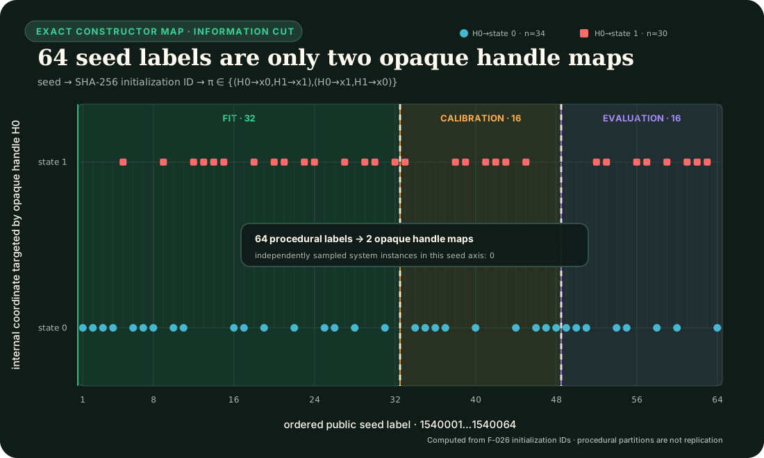
The plotted points are computed from the checked-in initialization-ID and opaque-permutation functions. The colored regions show the access cut; they do not add independent system variation.
The two generic references become mature nulls only after trainable causal state-space and compact recurrent estimators are implemented against the same fixed-parameter packet schema, with no direct plant state, recipe or equation access. Their construction, selection, calibration, failures and fallbacks enter the resource ledger. A later confirmatory comparison needs independently generated held-out system instances and an outer system-family holdout; neither exists in the present five-world bank.
For that later design, the fixed primary endpoint families are mean property
log loss in nats and mean dimensionless decision loss. Coverage, selective
risk, reliability, compatible-vector coverage and the resource vector are
reported alongside them. The earlier Stage-3 wording grouped the two
candidate-versus-generic-null contrasts within each endpoint. The later
population contract supersedes that weaker boundary and uses the sequentially rejective procedure of
Holm (1979), bibliography key
holm1979sequential, once across all four fixed
endpoint-by-comparator hypotheses at familywise . Sample size must be powered before private
confirmation seeds are created; 16 public evaluation labels are not assumed
sufficient.
The closed machine form is
rsd-t02-stage3-design.json,
validated by
rsd-t02-stage3-design.mjs.
Prospective system population and outer-family boundary
The information cut above remains valid, but it is not a population design. The next contract uses the following nesting, from inferentially broad to repeated measurement:
A procedural seed is only a replay key. A family is one frozen equation template plus a declared parameter distribution. An instance is one accepted parameter vector drawn independently from that family; it is the unit for a fixed-family estimand. Episodes, rows, property coordinates, solver refinements and noise realizations remain nested measurements and never increase the reported independent .
This distinction also invalidates a tempting reuse of the current packet. Its nine O0 executions cross , while its 26 O1 executions hold . One population instance must bind one parameter vector—including one time constant—across every episode. The old mixed- packet remains a construction-conformance artifact; a population packet must be regenerated per fixed parameter vector.
The first defensible claim mode is a fixed finite family panel. Visible development families and separately sealed outer-confirmation and outer-transfer families are split by structural lineage, not by recipe label or instance. Related equations, derivations, code siblings and full-panel- equivalent recipes share a leakage group and cannot cross partitions. An outer result therefore generalizes only to the prospectively frozen weighted panel, not to arbitrary future mechanisms. A family-superpopulation claim requires a separate frozen probabilistic family grammar and powers on independently drawn families or lineages.
For coordinate , instance , family and arm , first aggregate the coordinate loss inside the instance,
Then form the equal-family weighted contrast
Resampling occurs over instances within the fixed families; rows are never resampled as independent systems. The prospective power artifact must freeze the smallest effect of interest, alpha, power, family heterogeneity, family and instance counts, abstention coverage, failure disposition and the calculation implementation hash before private responses. The experiment-level success rule applies Holm's procedure across all four fixed endpoint-by-comparator hypotheses at ; controlling two contrasts separately inside each endpoint would not close the cross-endpoint multiplicity boundary.
For equal retained counts in each of fixed families, first derive the minimum effective count for one lower-tail contrast:
Here is the development-evaluation variance of the paired system-instance contrast in family , is the minimum relevant improvement magnitude in the endpoint unit, and is target power. The term protects the most conservative first Holm step.
If is the prospective probability of pre-response invalid generation and is the registered experiment-level retention assurance, the plotted planned count is instead
The Bonferroni allocation on the right guarantees at least retention assurance across the family strata without assuming their attrition events are independent. Runtime failures retain their registered in-denominator penalty. The support-coverage floor remains a separate gate and is not silently converted into another sample-size multiplier.
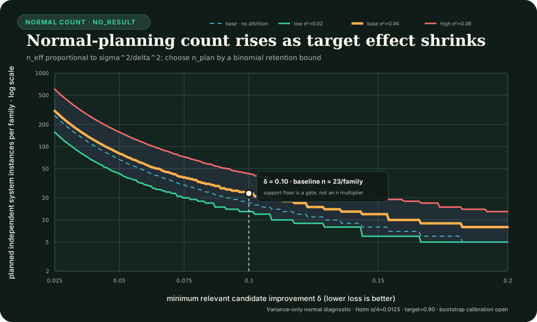
The figure is a sensitivity map, not a power result. Its variance profiles are illustrative, so it cannot freeze a sample size. The checked-in calculator requires a development-evaluation variance-artifact hash and exposes every unit, approximation, attrition rule and blocker. A syntactically valid hash does not verify the artifact bytes, role or review, so the calculator always keeps the power-plan release gate open until those bindings are independently validated. The normal calculation also does not establish power for the final bootstrap- analyzer: zero-standard-error bootstrap resamples create a data-dependent lower bound
where is the registered resample count and is the number of zero-standard-error resamples conservatively counted as extreme. The analyzer records this bound for every hypothesis and closes its resolution gate only when it can reach the first Holm threshold. A future frozen power artifact must therefore simulate the pilot transcripts through the exact analyzer; variance alone is insufficient.
Synthetic transcript calibration of the exact analyzer
The public diagnostic now performs that simulation step for four declared synthetic scenarios without treating the resulting frequencies as scientific power. For events in Monte Carlo replicates it reports the smoothed point diagnostic
The point smoothing and interval have different jobs. The Wilson score interval is computed for the observed binomial count ; applying Wilson to the artificial pair would give the wrong coverage target and can exclude zero even when a deterministic hostile produces no events.
The generated unit identity uses a DGP-only fingerprint. It binds scenario baselines, attrition, failure probabilities, contrast means and covariances, the simulation key and registered family order. Confidence level, total replicate ceiling, bootstrap count, alpha and endpoint penalties remain in the full configuration/report identity but do not reorder a common generated prefix or change its finite-bootstrap point decision.
The canonical configuration uses and . Its declared synthetic null yields 6 any-rejection events, while the declared minimum-relevant-effect scenario yields 55. The null Wilson Monte Carlo interval, --, spans the reference; the alternative interval, --, is far below the illustrative target. The two two-instance hostiles each fail the analyzer's bootstrap-resolution gate in all 99 replicates. This rejects plan acceptance; it does not estimate future model power.
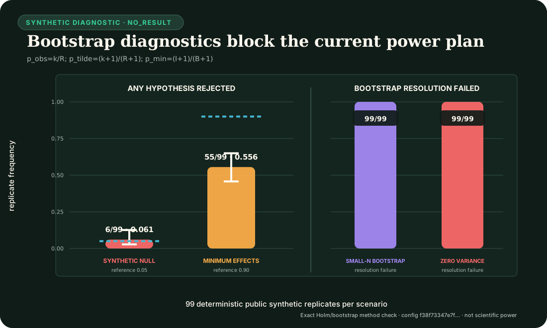
The executable contract is
rsd-t02-pilot-transcript-calibration.json,
implemented by
rsd-t02-pilot-transcript-calibration.mjs.
Closure is narrow: reviewed real pilot bytes and role, an analyzer release hash,
jointly frozen effects, target, resampling key and failure penalties, and an
accepted planned-count calibration remain open.
The causal-memory coordinate is not primary-scorable in this first population design because the current family bank contains no valid memory-negative lineage. It can become primary only after both values have prospective, lineage-diverse coverage. Outer family templates and truth remain encrypted or evaluator-custodied until the model, calibration, thresholds, analyzer, resource caps and power plan are frozen. A bare public hash is a commitment, not secrecy for a small family search space.
The closed prospective machine form is
rsd-t02-population-design.json,
validated by
rsd-t02-population-contract.mjs.
Exact public fixed-instance construction
The public family registry currently contains the five named equation families only. Four generator-conformance coordinates are crossed with every family, producing 20 metadata artifacts. This count tests deterministic construction; it is not a powered sample size.
For family , draw index , parameter key , and HMAC attempt , let
hashes the ordered scientific family definitions only; coverage policy, custody state, packet metadata and generator authority are excluded. binds the selected family, including its declared equation- template digest. is committed replay material rather than a secret. The sole sampled parameter is an integer time constant
With possible integers and
the generator rejects before applying modulo reduction, then uses
The complete parameter document stores exact numerator, denominator and unit objects. Its digest, the fixed nuisance-interface digest and complete certificate-set digest, including the equation-template digest, enter the canonical system identity. The full registry, population-design bytes and model-source bytes remain separate provenance bindings. The draw index is recorded in the receipt but not in that identity. Every generated packet lists the same parameter digest and on all 26 unique episodes. A distinct episode-protocol digest binds every schedule, the horizon, integration step, output rate, input bounds, units and interpreter semantics into the packet ID without contaminating the system ID. The generator packet itself contains no trajectories or policy response. A separate fixed-instance conformance runner now materializes its 26 trajectories and causal view. An additive overlay binds a content-addressed 26-projection abstention bundle, executes it in a fresh restricted child, semantically replays the nine responses, and durably resumes an owner-bound fixed-instance ledger. A compact population runner traverses all 20 unique public instances and receipts 520 episodes, 799,240 transcript rows and 180 arm invocations. The integrated execution release composes both layers: one identity-keyed durable instance directory per system and one bounded outer record only after its nine-arm summary is complete and current. Restart tests cover the post-instance/pre-outer crash window and full-panel reopen without duplicating a scientific unit. The outer records contain no endpoints or causal payloads, and the release still does not execute the trained candidate or null policies.
The coverage function counts distinct structural lineages per property value, collapsing the full-panel-equivalent I1-FFL and affine high-pass siblings into one lineage. The frozen minimum is two:
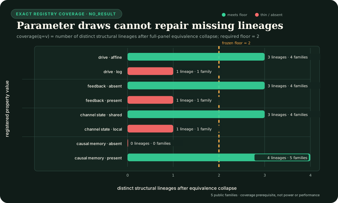
log-fold, feedback-present and channel-local-present each have one lineage;
memory-negative has zero. More draws from the current equations cannot close
those structural gaps. The closed machine artifacts are the
family registry,
instance plan, and
generator.
Generic-null maturity is a state machine
The executable B-STATE-SPACE and B-RECURRENT policies in the older
35-projection construction bank remain fixed level-one references. Separate
deterministic trainable implementations now provide a causal latent state-space
prototype and a compact GRU-style prototype. They consume the fixed-instance
causal view only through a post-validation adapter and occupy level two; they
do not replace the older policy responses. The maturation sequence is:
- fixed conformance reference;
- trainable public prototype;
- fit-frozen development estimator;
- calibrated development comparator;
- confirmation-frozen mature null; and
- confirmation-evaluated run state.
Only level 5 satisfies the population gate. Both current trainable prototypes
are at level 2. They emit normalized value posteriors for all three primary
coordinates, identifiability probabilities, one coherent joint posterior,
support status, a deterministic decide-or-abstain action, reason codes and a
typed work ledger, but their probabilities are uncalibrated and their models,
resource caps and source/runtime identity are not comparison-frozen. The
machine implementations are the
prototype module,
post-validation adapter,
and
maturation design.
For instance and property , a prospective common objective family is
is the trainable parameter vector, indexes system instances, and indexes active property coordinates. Let be the finite active joint property-vector domain. For each , the joint posterior is normalized by , while the evaluator supplies a nonempty set of compatible vectors. Zero posterior mass on all of gives an infinite negative log-mass penalty.
is certified identifiability and its predicted probability. If , is the unique property truth and a normalized posterior over the registered values of coordinate . If , is not required and the masked expression is defined as . and are respectively the auxiliary causal-prediction loss and frozen regularizer. They, BCE, CE, and the log-mass term are normalized to dimensionless quantities.
The fit-only training weights satisfy and ; they are not the common endpoint-aggregation weights , , which freeze before development evaluation. The coefficients and are dimensionless and selected inside fit. Predictive horizon, optimizer and stopping rule remain fit-only choices, while the deterministic trial tie-break freezes before any trial outcome exists. Until the causal-memory activation condition passes, and span the three primary coordinates only; activating the fourth coordinate requires a new contract version, head and calibration.
The exact six-level status, freeze order, common resource requirements and
three separate gate scopes are frozen in the
null-maturation design.
The two trainable-prototype gates and the parameterized isolated durable runner
gate are satisfied; seven intrinsic null-maturity gates remain open. Two of ten
comparison-release gates—the registry and generator—are also satisfied; the
measured-energy meter gate is
conditionally applicable only when an energy claim is requested. It is not
counted among the 20 mandatory gates for a non-energy comparison. The current
non-energy total is therefore five satisfied and 15 open. Affected fitting
remains blocked by incomplete lineage coverage, absent sealed outer-family
templates, and the absent instance-level fit/calibration/development-evaluation
assignment. The exact local runtime closure for the promoted infrastructure
gate is recorded in the
parameterized runner release.
Calibration and abstention
Probability quality is evaluated with logarithmic loss as a proper scoring
rule in the sense reviewed by
Gneiting and Raftery (2007),
bibliography key gneiting2007scoring. The
separate decision loss below encodes this fixture's abstention costs; it is not
silently folded into calibration.
For property coordinate , let be the set of values compatible with the registered observation packet and define
When , let denote the unique element of .
An arm returns a probability , a posterior over property
values, including posterior mass on that unique compatible
value, and either decide or abstain. With probabilities clipped at
, the calibration loss in nats is
When , the final masked term is defined to be exactly zero; and are not evaluated.
The decision loss is dimensionless:
Coverage, selective risk and reliability remain separate. Sensitivity analyses later vary the identifiable-case abstention cost to and ; they do not replace the primary loss.
The fast boundary layer needs the right norm
The source-qualified stratum uses the nondimensional input-degradation model
with , , , and . The scaled member uses , and .
The primary finite-grid truth is
For this registered construction, the associated fast initial-value systems give
and a source-shaped finite- bound has the form
The protected construction does not infer this asymptotic statement from a finite sweep. It checks the declared generator and bound.
An RMS score measures something else:
The exact physical-time metric counterexample
has
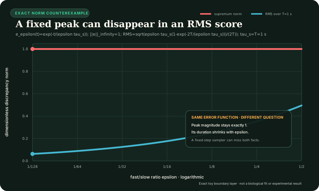
The figure is an exact toy norm comparison, not a biological fit or a run of the source-shaped generator.
Fast- and slow-time sampling
The protected grid freezes
The critical initial-layer time is
Every cell samples the union
The first grid resolves the shrinking boundary layer; the second retains the eight-second slow response. Deduplication leaves at most 1,537 paired rows per cell.
The floor stratum crosses three equation-defined models, seven epsilon values and five scale factors. Besides the singular system above, both controls share
The exact-equivariance control reports
Because the scaled member has and , its discrepancy is identically zero. The regular-perturbation control reports
Its scaled-versus-unscaled discrepancy is and therefore tends to zero. The three registered models are consequently:
- the source-shaped singular construction;
- an exact-equivariance zero-floor control; and
- a regular-perturbation control whose discrepancy tends to zero.
That is 105 public-development cells and at most 161,385 paired rows. RMS is diagnostic only and cannot establish or refute the supremum floor.
Information firewall
Every actionable arm receives only causal inputs, reported outputs, masks, opaque intervention commands, timestamps and units. Before the arm response is frozen it does not receive:
- recipe or equation identity;
- semantic state names or the hidden handle permutation;
- parameters or evaluator properties;
- future samples or future-derived normalization;
- the equivalence or separation certificate; or
- continuous evaluator truth.
The actionable registry has nine roles:
A-RAW;B-STATIC-DIV;B-STREAM;B-LOG-RATIO;B-DIFFERENCE;B-STATE-SPACE;B-RECURRENT;C-MECHANISM-BANK; andC-DUAL.
O-GRAPH is evaluator-only and excluded from parity, tuning, promotion and
resource rankings. Public source code does not create confirmation secrecy; a
claim-eligible run later needs separately committed sealed seed mapping and
custody.
Typed acquisition and computation cost
Do not collapse intervention access and execution into one score. Every arm retains at least:
- episodes and sample rows;
- serialized observation bytes and input commands;
- internal resets, freezes and output clamps;
- channel switches and state writes;
- scalar operations and transcendental evaluations;
- retained-state and parameter bytes;
- tuning trials and wall seconds; and
- later measured joules, when a calibrated physical protocol exists.
The foundation suggests future caps of one CPU thread, binary64 arithmetic, 16 retained scalars, 512 trainable scalars and 32 tuning trials. They are not active parity claims because actionable algorithms and a complete arm-level parity/resource ledger are absent.
Support and fail-closed cases
Each scientific case retains the six independent support axes already frozen for RSD-T01:
- input domain;
- transformation family;
- instrument range and temporal resolution;
- initialization;
- causal observation; and
- evaluation window.
Valid scientific hostiles include additive offset, near-zero input, clipping, hidden reset, future-aware normalization, channel-state contamination and boundary-layer censoring. Parser, checksum, order or unit failures remain malformed sentinels outside the scientific denominator.
Missing, duplicate, rejected or mixed-initialization transcripts force system abstention and remain visible. A fixed slow-time sampler that misses the protected fast layer is a scientific failure, not a missing-data deletion.
Current authority and kill rules
The machine registry states:
{
  "authority": "contract-foundation-only",
  "partition": "public-development",
  "information_cut_status": "registered-projection-no-secret-custody",
  "comparison_authority": false,
  "result_authority": "NO_RESULT"
}
The registry is the foundation authority, not the execution result. A separate
deterministic bounded public-development runtime now consumes the T02-MECH
registry to generate all O0/O1 construction episodes, enforce the policy
firewall and response commitment, reconstruct evaluator truth, retain typed
acquisition/construction/inference ledgers, and validate append-only resume.
Its additive Stage 2 commits all nine fixed whole-system policy-conformance
responses before evaluator access, with zero inactive placeholders. Every event
and analysis remains NO_RESULT; trained or
calibrated estimators, mature nulls, comparisons, claim eligibility, O2, T02-FLOOR
execution, confirmation, workstation measurement and energy conclusions are
absent.
The future T02 comparison is killed if any of the following occurs:
- step fit, recipe name or graph access supplies the primary answer;
- a declared separating intervention lacks a pairwise certificate;
- an arm is rewarded for guessing inside an observational equivalence class;
- privileged access is unequal or missing from the cost vector;
- RMS or a fixed slow grid substitutes for the registered supremum endpoint;
- a finite epsilon sweep is presented as proof of an asymptotic theorem; or
- a mechanism-specific bank cannot beat the generic state-space/recurrent null under the same projection and budget.
The current foundation and construction runtime can test equations, exact step matching, operational equivalence, registry closure, schedule semantics, abstention aggregation, replay integrity and temporal-grid coverage. They cannot support architecture superiority, natural-mechanism attribution, workstation readiness or energy efficiency.