- Status: frontier notation and experiment design; no result
- Audit: history-conditioned modular succession and priority effects
- Promotion boundary: this note creates no claim, principle, candidate, protocol, or fixture identifier
- Purpose: define fixed-task-and-eligibility order estimands, resource identities, causal-cut contrasts, endpoint units, multiplicity control, and kill boundaries before any large implementation is proposed
Scope
The mathematical question is whether a randomized sequence changes a final learned system after the presented task multiset, eligible module identity set, and all declared resources are held fixed. Realized active, consolidated, merged, or retired module state may differ and is an endpoint. The notation does not assume that an order effect exists or that any effect is ecological in mechanism.
Microbial abundance, model accuracy, allocated parameters, examples, seconds, bytes, and joules remain different quantities. No conversion among them is introduced here.
Indices, objects, and units
| Symbol | Definition | Unit |
|---|---|---|
| number of distinct task blocks and eligible module identities in the bounded design; initially | count | |
| paired admission-unit index, | count | |
| executing-module index when tasks and modules are evaluated separately | count | |
| sequence-position indices, each in | count | |
| paired random-seed index | count | |
| learning-method index | category | |
| endpoint index | category | |
| distinct mechanism-factor indices when used together | category | |
| frozen multiset of task blocks | set-valued | |
| checksummed task block with identity | data object | |
| eligible module identity paired with before randomization | typed identity | |
| frozen task/module admission unit | typed pair | |
| set of all permutations of identities | set-valued | |
| one randomized permutation in | dimensionless mapping | |
| paired admission-unit identity shown at sequence position | count | |
| vector of binary mechanism interventions | dimensionless vector | |
| complete learned and structural state for method after position | typed state | |
| trainable parameter state within | parameter vector | |
| router/admission state within | typed state | |
| optimizer state within | typed state | |
| replay or external learning-memory state within | typed state | |
| capacity-allocation state within | parameter/byte vector | |
| observed endpoint for one method, order, intervention cell, and seed | endpoint-specific | |
| seed expectation of under the frozen generator | endpoint-specific | |
| exogenous examples presented from task | count | |
| examples from task accepted by executing module | count | |
| optimizer-update applications to attributed to examples from under the frozen attribution rule | count | |
| total installed parameter-capacity ceiling | parameters | |
| maximum simultaneously active parameter ceiling | parameters | |
| peak live attributed storage | bytes | |
| elapsed wall time from the registered run start | seconds | |
| calibrated externally measured run energy at the declared boundary | joules | |
| mean measured power over a declared interval | watts |
Every typed state is serialized or hashed at each task boundary. A variable that affects later updates but is absent from is an unmeasured shared state and invalidates the corresponding causal cut.
Fixed-task-multiset and module-eligibility identity
For the initial design, freeze a one-to-one admission map before order assignment and define . Each pair appears exactly once. A valid permutation satisfies
as a bijection, and therefore
where denotes multiset union. Equivalently, for every identity ,
Here is a dimensionless indicator. If a later design repeats blocks, the right-hand side becomes a frozen multiplicity that is identical for every order. Adding or deleting a presented task, eligible module identity, initialization image, example, label, augmentation, or response opportunity violates the order estimand. Realized activation, consolidation, merge, or retirement does not violate it; those states remain measured outcomes.
Let be the stored initialization image for paired module and seed . It is drawn before is assigned, so
for all compared orders and . Every other random stream is keyed by its typed identity and paired seed rather than by global call order. Otherwise a permutation could change initialization, dropout, augmentation, router, or fault draws and the contrast would not isolate order.
Let denote the frozen stream bundle keyed by admission unit , paired seed , stream type, and within-identity draw index. A sequence position selects that identity's bundle; it does not create a new position-keyed bundle.
The method-specific state transition is written abstractly as
where is the frozen transition implementation and is the paired random-input bundle for the identity occupying position . Position-indexed exogenous disturbances are prohibited unless they are a separately registered, randomized factor. This notation permits parameters, routers, optimizer moments, replay, and structure to carry history; it does not require all methods to contain every component.
Exposure, capacity, optimizer, evaluator, and budget identities
Exogenous exposure
For each task , let be the frozen checksummed sequence of examples, labels, augmentations, and interaction outcomes. Exogenous parity requires
for every method and order in a matched comparison. The equality is in counts and content: equal counts with different examples are not equal exposure.
Routed acceptance may be an endogenous mechanism. The accepted-exposure ledger therefore retains both task identity and executing-module identity . Define the task-total accepted count and its dimensionless exposure ratio as
The ratio can exceed one only when the registered method duplicates or fans out one presented example to more than one module; every duplicate remains charged. Module-total accepted exposure is
The exposure-equalizer intervention freezes the complete task-by-executing-module targets and such that
for every task , executing module , and evaluated order in that intervention level. Thus equal task totals cannot hide a different routing allocation. Mixed-task update attribution and any fan-out rule are frozen before order assignment. Rejected, downweighted, or duplicate work remains charged even when it is not applied as an update.
Let be module 's birth time in seconds from run start and let be the registered run duration in seconds. Its final wall-clock age is
The pre-instantiation cut sets all while freezing inactive state. The exposure equalizer changes the and matrices, not . This is why age and accepted exposure can be crossed independently.
Capacity
Let be parameters allocated to module at time , and let indicate that the module is active. Valid runs satisfy
and
for all measured . Every term is a parameter count. Storage for optimizer state, router state, replay, checkpoints, and metadata is counted separately in bytes; parameter count is not treated as bytes without the registered representation width.
For the position-blind reservation cut, frozen quotas obey
Unused reserved capacity cannot be borrowed. Otherwise the later order could change effective total opportunity while nominal capacity remained fixed.
Optimizer and evaluator
Let be all optimizer updates, including replay, router, consolidation, recovery, and failed-attempt updates. Let be evaluator calls. Within a method-specific order contrast,
for every compared and , unless a count is itself a declared endpoint under a common ceiling. If early stopping is allowed, unused budget is reported; it is not silently transferred to tuning.
Across different methods, the optimizer mechanism may differ. Equality then means equal allowed update, search, evaluator, precision, and stopping budgets, not pretending that EWC, OGD, replay, PBT, and ordinary SGD execute identical operations. Method-specific work remains visible in the complete ledger.
Complete budget vector
Let be total presented exposure. Total accepted task-by-module exposure is
Let and be forward- and backward-evaluation counts, and let , , and be attributed read, written, and peak-live byte counts. Let be summed provisioned worker time in seconds, be elapsed run time in seconds, and be calibrated external energy in joules. and retain the definitions above.
Define
The first six entries are counts; the next three are bytes; and are seconds; is joules. This vector is never summed directly. Paired order arms require componentwise equality within frozen tolerances or are compared on a preregistered Pareto frontier.
Mean measured power is derived only when a calibrated energy interval of duration seconds exists:
Because , is in watts. Operations, parameters, or bytes cannot replace in this equation.
Potential outcomes and order estimands
For endpoint , method , intervention vector , and order , define the seed expectation
where the expectation is over the frozen seed generator, not over all possible tasks or machines.
Pairwise order effect
For two preregistered orders and , the controlled order effect is
Its unit is the endpoint unit. A positive value is beneficial only when higher values of endpoint are defined as better. Costs and errors retain their natural lower-is-better direction rather than having signs silently reversed.
The paired estimator over seeds is
where is a dimensionless seed count.
Order-distribution sensitivity
Let . The permutation-average endpoint is
The between-order variance is
This is the finite-population variance for an order drawn uniformly from all permutations. If only orders are sampled uniformly without replacement, the preregistered sample estimator uses denominator and reports its sampling uncertainty; it is not silently substituted for the complete enumeration. If is a dimensionless score, the variance is squared score units. The order range is
in the endpoint unit. The range is descriptive and selection-biased as an estimate of a future best order; it cannot replace simultaneous pairwise intervals.
Position effect
For task identity and position , define
The position contrast
compares the same task at two positions averaged over all orders of the other tasks. It is not an “early-arrival law” unless it replicates across protected task families and survives the mechanism cuts.
For a plot or table that compares every position with the task's mean over positions, define
Thus . If the only changed factor is the capacity-reservation cut, its position-specific interaction is
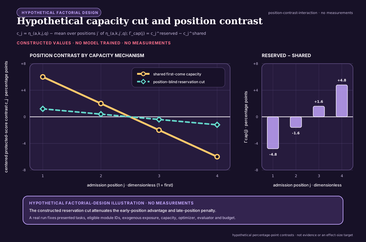
The figure is an algebraic reading aid. It substitutes constructed percentage-
point contrasts for and plots their constructed difference as
. The values are not measurements,
estimates, predictions, recommended effect sizes, or evidence that a capacity
mechanism exists. Its editable specification is the
history-conditioned-position-contrast entry.
Optimized-order advantage
Let be a frozen order-selection algorithm, let be its selected order using discovery information only, and let be the uniform distribution over admissible orders. The held-out optimized advantage is
The quality contrast is incomplete until the order optimizer's pilot examples, similarity or curvature measurements, candidate sequences, evaluator calls, failed runs, bytes, seconds, and joules are appended to . Selecting the observed maximum from confirmation orders is not and is not a valid optimized-order estimate.
Factorial mechanism estimands
Define the binary intervention vector
where is the natural-history level and is the causal-cut level defined in the audit. Let denote all factors except mechanism .
For one order , the controlled main contrast of mechanism at fixed is
The order-by-mechanism interaction for two orders is
has the endpoint unit. If cutting a path reduces an order contrast toward zero, that is evidence that the measured effect depends on the cut under the frozen design. It is not proof that mechanism is the only mediator.
For distinct mechanisms and , the two-factor interaction at one order is the inclusion--exclusion contrast
where the two subscripts give and all remaining factors are fixed. Higher-order interactions use the same inclusion--exclusion rule.
Decomposition limits
The factorial is randomized, but a unique additive causal decomposition is not generally available because:
- capacity changes which exposures are accepted;
- exposure changes optimizer and shared-state trajectories;
- shared state changes routing and therefore capacity demand;
- facilitation changes both information and subsequent work;
- lock-in changes the set of later admissible states; and
- nonlinearity allows higher-order interactions.
Consequently,
in general. The right side also depends on the levels at which the other factors are fixed. “Percent mediated” is not reported unless a separate causal model supplies and defends the required cross-world assumptions.
Ordinary-scheduling negative control
Let denote a task job that consumes the same declared compute and I/O but does not update parameters, routers, optimizer state, replay, normalization, or structure. Let be its completion order under scheduler input . Scheduling may change a service endpoint such as latency in seconds.
Separately, let be the complete checksummed learned update record produced for task . Apply all records after job completion in one canonical order to obtain
If and all final capability endpoints are identical across input permutations while only differs, the detected effect is ordinary scheduling under this control. If update records themselves depend on the live history, canonical replay is diagnostic rather than an oracle; that dependence must be attributed to one or more serialized state paths.
Learning endpoints
Assume higher task score is better. Let be task 's held-out score immediately after its acquisition block, and let be its score after all blocks at the frozen retention horizon. Both retain the declared task score unit.
Backward transfer is
Positive values indicate improvement and negative values indicate forgetting. The nonnegative forgetting magnitude is
Let be the preregistered protected score floor for task . The protected shortfall is
This has the score unit and cannot be cancelled by high performance on another task. The worst-task score is
For newcomer task , let be a frozen competence threshold and let be the first accepted-example count at which the threshold is met and remains met for the frozen confirmation window. If the threshold is never met, is right-censored at the task budget rather than deleted. Forward facilitation is evaluated through this sample-complexity endpoint and a matched no-history baseline, not through final score alone.
Structural and routing endpoints
Let be the fraction of routed load assigned to executing module at time , with
when at least one module is eligible. Router entropy is
in nats when the natural logarithm is used. Terms with contribute zero. Low entropy is not by itself specialization or quality.
For a frozen task-by-module evaluation matrix , where row is task identity and column is module identity, define a dimensionless specialization contrast for module as
where is the task attaining the maximum under a frozen tie rule. This metric is meaningful only if uses a common dimensionless score. If tasks have different native units, their raw matrix is reported and no such subtraction is allowed.
Admission time, commitment time, unlock count, retirement count, allocated capacity, accepted load, dropped load, and lineage remain separate endpoints. An expert label or high does not prove independent function, causal necessity, or efficient routing.
Service and lifecycle endpoints
If predictions are due and are correct, current, integrity-valid, and within the frozen deadline, accepted service is
a dimensionless fraction. Missing, late, stale, duplicated, and inaccurate predictions remain separate counts before aggregation.
Latency for due item is completion time minus original due time, in seconds. Every due item remains in the denominator; missing completions receive the preregistered right-censor value. p50, p95, and p99 are reported with the exact quantile convention.
The mandatory result is a vector,
The entries have different units and are not averaged. Method dominates method only under preregistered direction and relevance margins, with no protected endpoint worse and at least one endpoint materially better.
Multiplicity and uncertainty
Let be the frozen family of primary order, method, and order-by-mechanism contrasts. Its membership is committed before confirmation outcomes are opened.
For randomization inference, compute one test statistic for each and, under the registered treatment re-randomizations, use the maximum absolute standardized statistic
The empirical distribution of supplies family-wise adjusted decisions and simultaneous intervals. If that procedure is computationally unavailable, Holm's step-down correction is the fallback. Unadjusted effect estimates and intervals remain visible, but they cannot carry the confirmatory decision.
Seeds are paired experimental units only for the generator they instantiate. Tasks, orders, endpoints, or repeated checkpoints from one run are not treated as independent sample-size multipliers. Generalization to a task population or machine population requires corresponding sampled levels and a second-family or second-machine replication.
The minimum relevant effect is declared in endpoint 's native unit. “Statistically nonzero” without crossing does not keep the frontier alive.
Dimensional analysis checklist
- Task scores may be dimensionless proportions or native score units; the unit is declared before subtraction.
- Counts of examples, updates, parameters, modules, calls, and operations are dimensionless counts with different meanings and are not interchangeable.
- Storage and traffic are bytes; parameter counts become bytes only after representation width and metadata are included.
- Latency, worker time, and wall time are seconds but have different boundaries and remain separately named.
- Energy is joules and power is joules per second, or watts.
- Throughput is accepted items per second and is not an energy efficiency.
- Quality per joule is reported only beside its raw quality and energy components at matched task, quality floor, horizon, and boundary.
- Ecological abundance and artificial router load are not assigned a common unit merely to make an analogy.
Testable predictions
These are preregistrable hypotheses, not findings:
- In high-overlap task strata, the capacity reservation cut yields opposite in sign to the natural order contrast if incumbency is carried by capacity pre-emption.
- If shared-state modification is a carrier, the magnitude of decreases when while private post-acquisition scores remain within their non-inferiority margins.
- If typed facilitation improves newcomer acquisition, setting increases the newcomer threshold count or right-censoring rate without a corresponding change under the sham-only scheduler control.
- If lock-in is useful rather than merely persistent, the irreversible arm improves protected delayed outcomes after the inducing module is removed and remains non-dominated after checkpoint, unlock, migration, and recovery costs enter .
- If the effect is ordinary continual-learning interference, replay, EWC, or OGD matches the complete frontier without module-birth factors.
- If the effect is curriculum selection, a held-out optimized order yields the same frontier after its search budget is charged.
- and the sign of position contrasts vary with feature overlap, readout conflict, horizon, and method; no universal early/late rule is predicted.
Numerical and contract checks
- Every stored permutation is a bijection and has the same task-multiset and eligible-module-set digests.
- Every task identity has identical exogenous example and update opportunity digests across orders.
- Capacity inequalities hold at every event, not only at final state.
- Every shared-state reset restores the same checksummed boundary image while retaining only the explicitly exempt private state.
- Sham facilitation payloads match byte count, availability time, parser work, and transport work, and are provably answer-free.
- Canonical replay applies exactly the same update-record multiset in the same canonical order for every scheduling control.
- Invalid, missing, censored, timed-out, and resource-exceeded runs remain in result tables and multiplicity families.
- The full budget vector is reconstructed from raw events before any method comparison.
- Half-precision, quantized, sparse, or parallel execution receives its own parameter, byte, work, and energy accounting; nominal operation equality is insufficient.
- No equation in this note authorizes a scientific, performance, or energy result before a registered executable package and sealed execution exist.
Kill boundary
This mathematical contract supplies no residual architecture contribution if:
- for every protected primary contrast on both task families, the registered simultaneous interval lies wholly inside ; the unobserved population condition is the corresponding no-effect region, not an executable decision rule;
- canonical replay or the non-learning scheduler reproduces the effect;
- equal age plus equal accepted exposure removes it;
- no randomized causal cut changes it on fresh seeds;
- a complete conventional null is non-inferior at lower or equal lifecycle cost;
- results depend on selecting the best confirmation permutation;
- protected-task harm or resource ceilings are violated; or
- the second task family or machine replication fails.
Passing these equations and checks would justify evaluating evidence. It would not by itself establish a biological equivalence, universal mechanism, or novel architecture.